Principal Component Analysis

Performs principal components analysis (PCA) on a xyz numeric data matrix.

# S3 method for xyz
pca(xyz, subset = rep(TRUE, nrow(as.matrix(xyz))),
                 use.svd = FALSE, rm.gaps=FALSE, mass = NULL, ...)

# S3 method for pca
print(x, nmodes=6, ...)

Arguments

xyz	numeric matrix of Cartesian coordinates with a row per structure.
subset	an optional vector of numeric indices that selects a subset of rows (e.g. experimental structures vs molecular dynamics trajectory structures) from the full xyz matrix. Note: the full xyz is projected onto this subspace.
use.svd	logical, if TRUE singular value decomposition (SVD) is called instead of eigenvalue decomposition.
rm.gaps	logical, if TRUE gap positions (with missing coordinate data in any input structure) are removed before calculation. This is equivalent to removing NA cols from xyz.
x	an object of class pca, as obtained from function pca.xyz.
nmodes	numeric, number of modes to be printed.
mass	a ‘pdb’ object or numeric vector of residue/atom masses. By default (mass=NULL), mass is ignored. If provided with a ‘pdb’ object, masses of all amino acids obtained from aa2mass are used.
...	additional arguments to fit.xyz (for pca.xyz) or to print (for print.pca).

Note

If mass is provided, mass weighted coordinates will be considered, and iteration of fitting onto the mean structure is performed internally. The extra fitting process is to remove external translation and rotation of the whole system. With this option, a direct comparison can be made between PCs from pca.xyz and vibrational modes from nma.pdb, with the fact that $$A=k_BTF^{-1}$$, where \(A\) is the variance-covariance matrix, \(F\) the Hessian matrix, \(k_B\) the Boltzmann's constant, and \(T\) the temperature.

Value

Returns a list with the following components:

L

eigenvalues.

U

eigenvectors (i.e. the x, y, and z variable loadings).

z

scores of the supplied xyz on the pcs.

au

atom-wise loadings (i.e. xyz normalized eigenvectors).

sdev

the standard deviations of the pcs.

mean

the means that were subtracted.

References

Grant, B.J. et al. (2006) Bioinformatics 22, 2695--2696.

Author

Barry Grant

See also

pca, pca.pdbs, plot.pca, mktrj.pca, pca.tor, project.pca

Examples

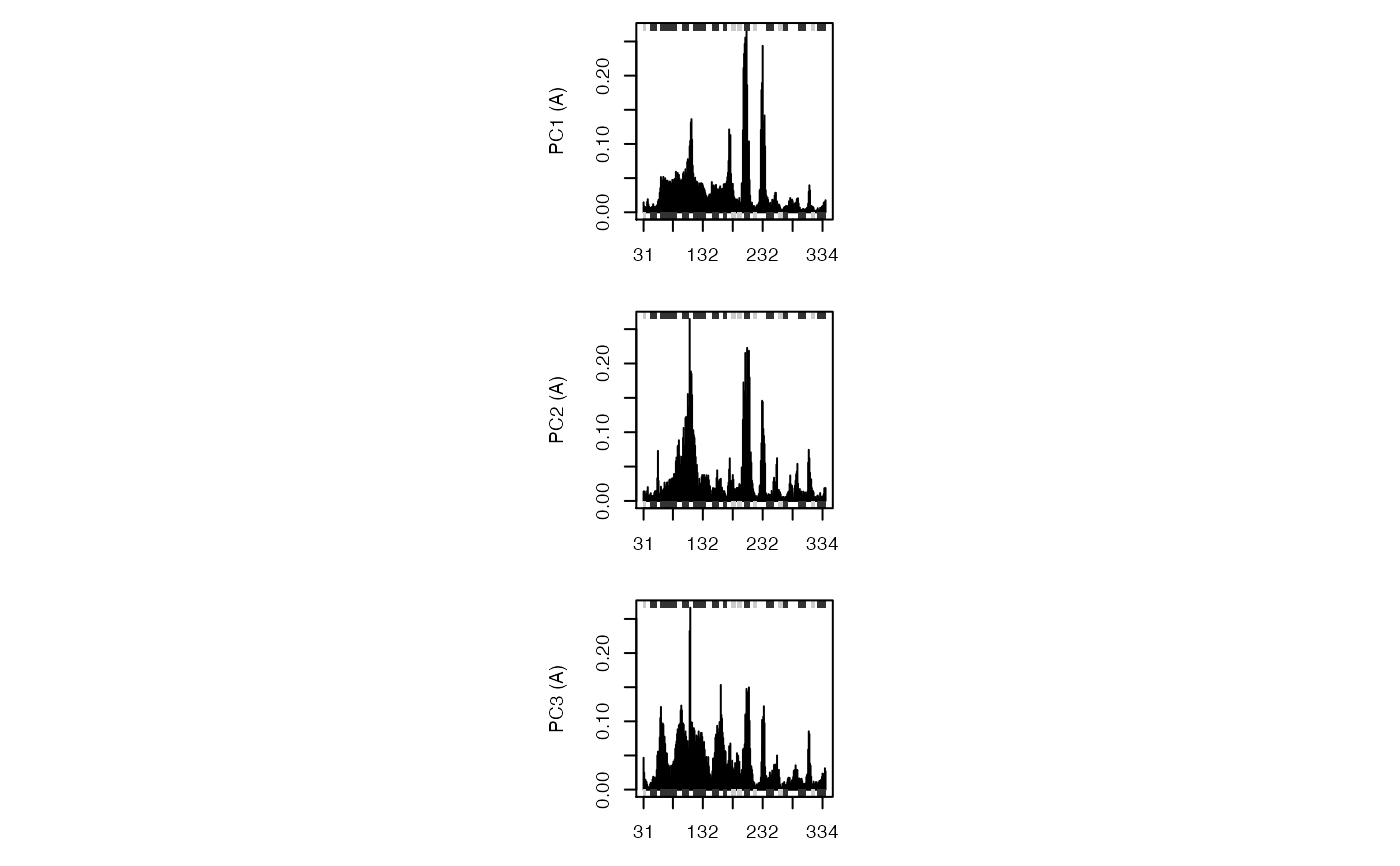
if (FALSE) {
#-- Read transducin alignment and structures
aln <- read.fasta(system.file("examples/transducin.fa",package="bio3d"))
pdbs <- read.fasta.pdb(aln)

# Find core
core <- core.find(pdbs, 
                  #write.pdbs = TRUE,
                  verbose=TRUE)

rm(list=c("pdbs", "core"))
}

#-- OR for demo purposes just read previously saved transducin data
attach(transducin)

# Previously fitted coordinates based on sub 1.0A^3 core. See core.find() function.
xyz <- pdbs$xyz
                
#-- Do PCA ignoring gap containing positions
pc.xray <- pca.xyz(xyz, rm.gaps=TRUE)
#> NOTE: Removing 49 gap positions with missing coordinate data
#>       retaining 305 non-gap positions for analysis.

# Plot results (conformer plots & scree plot overview)
plot(pc.xray, col=annotation[, "color"])

# Plot a single conformer plot of PC1 v PC2
plot(pc.xray, pc.axes=1:2, col=annotation[, "color"])

## Plot atom wise loadings
plot.bio3d(pc.xray$au[,1], ylab="PC1 (A)")

# \donttest{
# PDB server connection required - testing excluded

## Plot loadings in relation to reference structure 1TAG
pdb <- read.pdb("1tag")
#>   Note: Accessing on-line PDB file
#> Warning: /var/folders/xf/qznxnpf91vb1wm4xwgnbt0xr0000gn/T//Rtmp9oBdbc/1tag.pdb  exists. Skipping download
ind <- grep("1TAG", pdbs$id)             ## location in alignment

resno <- pdbs$resno[ind, !is.gap(pdbs)]  ## non-gap residues
tpdb <- trim.pdb(pdb, resno=resno)

op <- par(no.readonly=TRUE)
par(mfrow = c(3, 1), cex = 0.6, mar = c(3, 4, 1, 1))
plot.bio3d(pc.xray$au[,1], resno, ylab="PC1 (A)", sse=tpdb)
plot.bio3d(pc.xray$au[,2], resno, ylab="PC2 (A)", sse=tpdb)
plot.bio3d(pc.xray$au[,3], resno, ylab="PC3 (A)", sse=tpdb)
par(op)
# }

if (FALSE) {
# Write PC trajectory
resno = pdbs$resno[1, !is.gap(pdbs)]
resid = aa123(pdbs$ali[1, !is.gap(pdbs)])

a <- mktrj.pca(pc.xray, pc=1, file="pc1.pdb",
               resno=resno, resid=resid )

b <- mktrj.pca(pc.xray, pc=2, file="pc2.pdb",
               resno=resno, resid=resid )

c <- mktrj.pca(pc.xray, pc=3, file="pc3.pdb",
               resno=resno, resid=resid )
}

detach(transducin)