Introduction to Ensemble Difference Distance Matrix (eDDM) Analysis
Barry J. Grant, Lars Skjærven, and Xin-Qiu Yao
2020-09-14
Bio3D_eddm.spin.RmdBackground
The ensemble difference distance matrix (eDDM) analysis is a computational approach to comparing structures of proteins and other biomolecules(Grant, Skjaerven, and Yao 2020). It calculates and compares atomic distance matrices across large sets of homologous atomic structures to help identify the residue wise determinants underlying specific functional processes. The approach supports both experimental and theoretical simulation-generated structures. A typical eDDM workflow includes:
- Collecting and preparing the structure set
- Grouping structures
- Calculating difference distance matrices and associated statistics
- Identifying and visualizing significant distance changes.
The approach is implemented in the Bio3D package, bio3d.eddm. It can be integrated with other Bio3D methods(Grant et al. 2006; Skjaerven et al. 2014) for dissecting sequence-structure-function relationships, and can be used in a highly automated and reproducible manner. bio3d.eddm is distributed as an open source R package available from: http://thegrantlab.org/bio3d.
Requirement:
The latest bio3d and bio3d.eddm are required. See the Installing Bio3D Vignette for more detail. Once installed, type the following command to start using the package (Note that the dependent bio3d package is loaded automatically):
library(bio3d.eddm)
Collecting and preparing the structure set
In this vignette, we will use G protein-coupled receptors (GPCRs) as an example to illustrate the eDDM approach. The embedded code below can be used to reproduce the results described in the associated paper(Grant, Skjaerven, and Yao 2020). Specifically, we will analyze structures of the beta adrenergic receptor (\(\beta\)AR).
Using the pre-assembled structure set
Users are recommended to use the dataset shipped with bio3d.eddm for just to reproduce the results described in this document. This dataset contains 20 pre-assembled \(\beta\)AR structures. However, to apply the approach to other systems, users need to prepare the structure set from scratch (see next subsection).
attach(gpcr)
Getting the structure set from scratch
In this subsection, the detailed procedure to prepare the pre-assembled “gpcr” dataset will be described.1 Similar steps are required preceding other Bio3D analysis methods, such as principal component analysis (PCA) and ensemble normal mode analysis (eNMA) (see relevant Bio3D vignettes).
For users who simply want to reproduce the analysis reported in this document, this subsection can be skipped.
Starting with the sequence of the human \(\beta\)-2 adregenic receptor (UNIPROT: P07550), we search the PDB database to find structures with the same or similar sequence to the query, using the BLAST method implemented in Bio3D.
The identified structures are sorted in the descending order of sequence similarity to the query. A similarity threshold (on the E-value) is required to cut the searching result and determine the structure set for subsequent analyses. The Bio3D function plot.blast() or simply plot() can help find a suitable threshold by examining the distribution of the similarity scores.
hits <- plot(blast, cutoff=301)
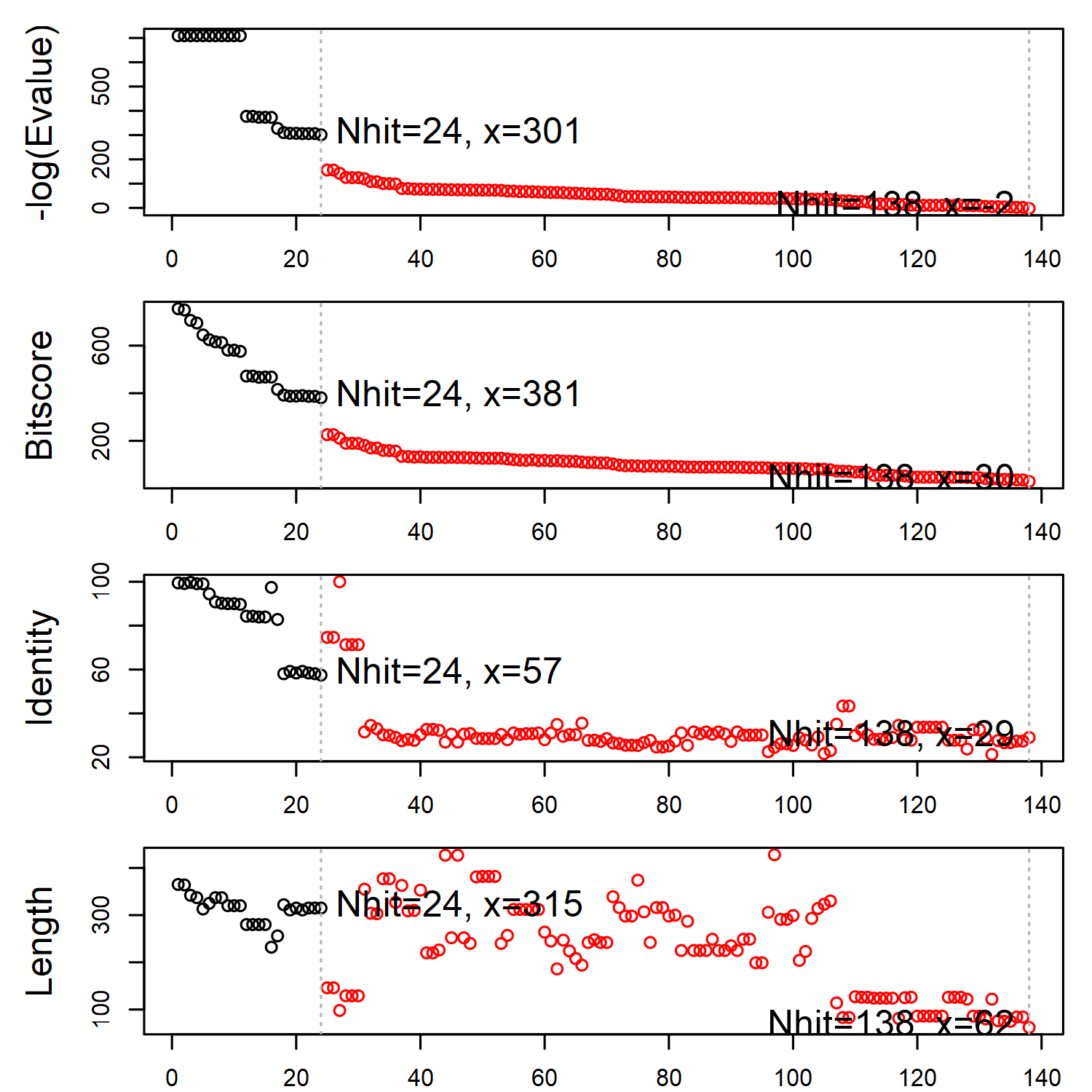
BLAST report regarding the search for beta adregenic receptor structures.
The structures can be further filtered by structural resolution (for crystallographic and cryo-EM structures). Such information can be automatically obtained using the Bio3D function, pdb.annotate().
annotation <- pdb.annotate(hits)
pdb.id <- with(annotation, subset(hits$pdb.id, resolution<= 3.5))
annotation <- subset(annotation, resolution <= 3.5)
Selected structrues are then downloaded through the Bio3D function, get.pdb(). The optional split=TRUE splits the downloaded files into individual chains to facilitate subsequent analyses.
files <- get.pdb(pdb.id, path="pdbs", split=TRUE)
All selected structures are aligned. This is to facilitate structural comparisons between “equivalent” or aligned residues.
pdbs <- pdbaln(files)
Grouping structures
The eDDM analysis compares structural ensembles under distinct ligation, activation, etc. conditions. At least two groups of structures are required. The grouping of structures can be either from available structural annotations (e.g., the ligand identity bound with each structure; such information is available in the above prepared annotation object) or from a structural clustering analysis. The latter approach is more general and requires minimal prior knowledge about the system. In the following example, we use PCA of the distance matrices (through the bio3d function, pca.array()) followed by a conventional hierarchical clustering in the PC1-PC2 subspace to get the intrinsic grouping of the \(\beta\)AR structures.
First, we need to update the aligned structures to include all heavy atoms. This is done by the bio3d function, read.all().
If the pre-assembled “gpcr” dataset shipped with the bio3d.eddm package is used through attach(gpcr), raw PDB data must be downloaded first.
get.pdb(pdbs$id, split=TRUE, path="pdbs")
pdbs.aa <- read.all(pdbs, prefix="pdbs/split_chain/", pdbext=".pdb")
Otherwise, if the dataset was rebuilt from scratch, type:
pdbs.aa <- read.all(pdbs)
In the following, we will calculate distance matrices, perform PCA, and cluster structures.
# Calculate distance matrices.
# The option `all.atom=TRUE` tells that all heavy-atom coordinates will be used.
dm <- dm(pdbs.aa, all.atom=TRUE)
# Perform PCA of distance matrices.
pc <- pca.array(dm)
## NOTE: Removing 178047 upper triangular gap cells with missing data
##       retaining 17578 upper triangular non-gap cells for analysis.
# See Figure 2. plot.pca.scree(pc)
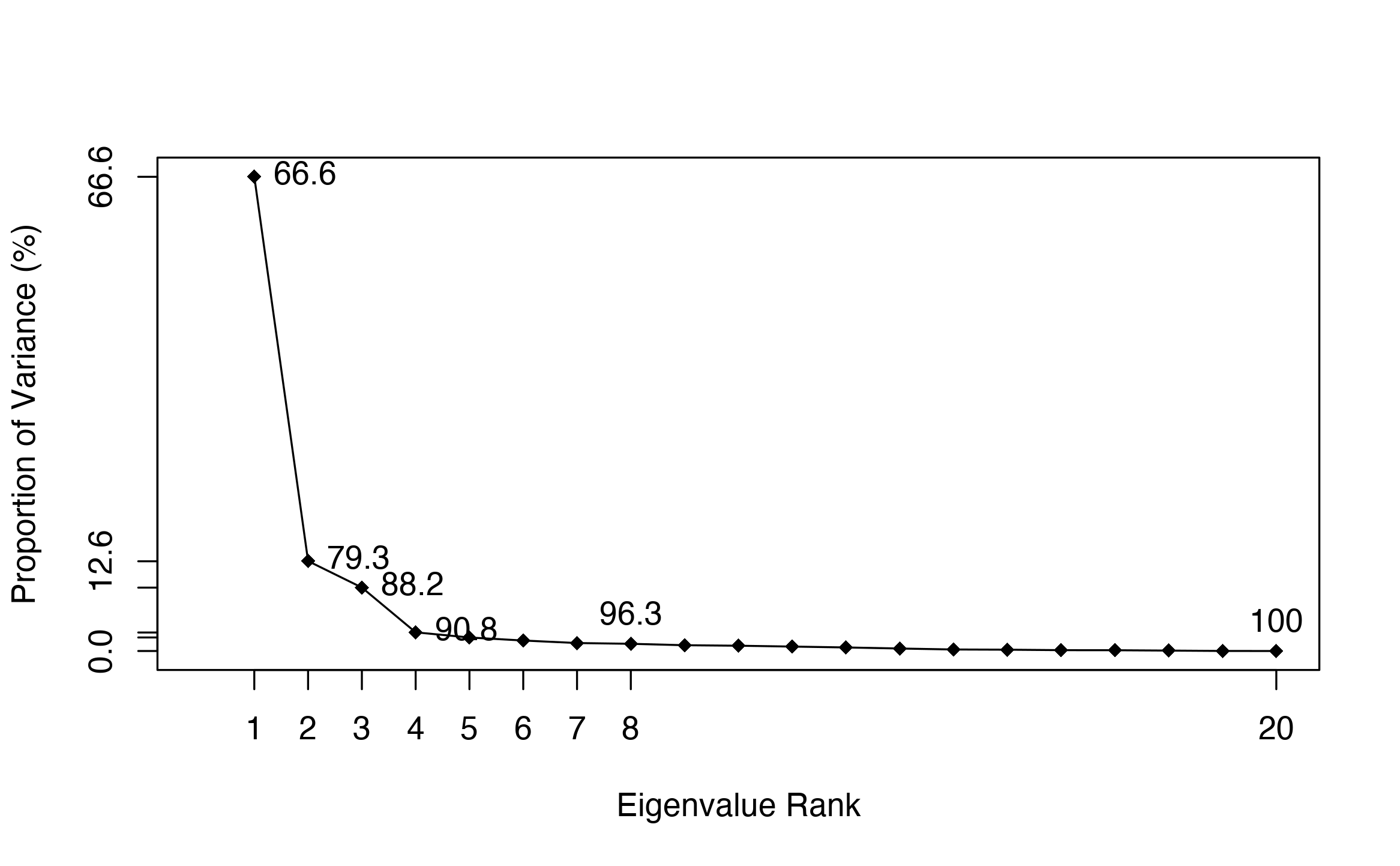
Scree plot of PCA. It indicates that the first principal component (PC1) is dominant over other PCs.
# Perform structural clustering in the PC1-PC2 subspace.
hc <- hclust(dist(pc$z[, 1:2]))
grps <- cutree(hc, k=3)
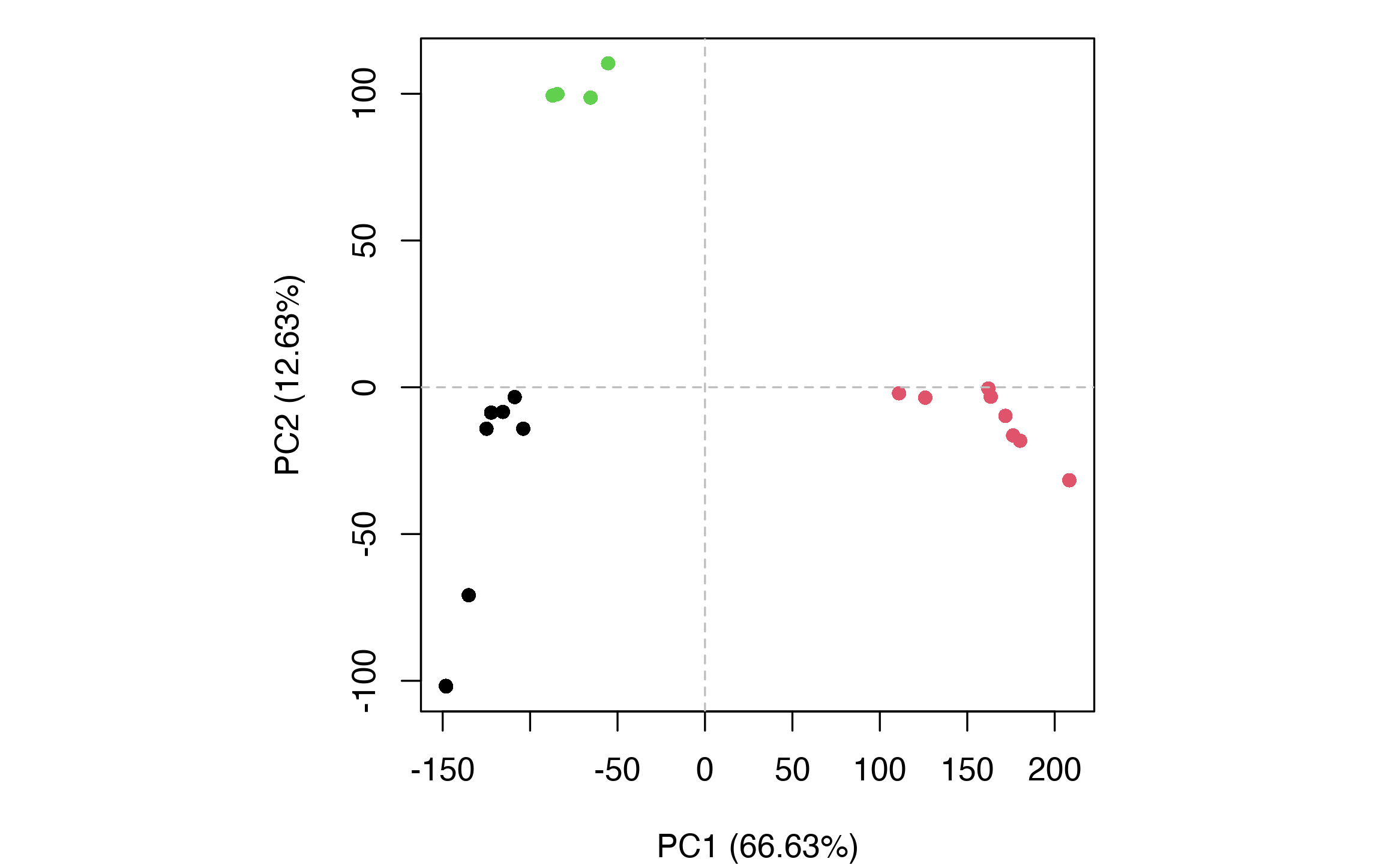
Conformer plot. Each point represents a structure with point color indicating the membership ID of the clustering. Three major clusters or groups are identified: Group 1 (black) representing inactive GPCR structures, Group 2 (red) representing active GPCR structures, and Group 3 (green).
Calculating difference distance matrices and associated statistics
The eddm() function calculates the difference mean distance between groups for each residue pair and statistical significance assessed using a two-sample Wilcoxon test. Long-distance pairs in all structures are omitted. This step is controlled by the mask option of the function. By default, the function uses mask="effdist", which calculates “effective” distances where changes for long-range residue pairs are scaled down to zero while changes involving short-range interacting residues are kept intact. This “mask” method is designed to assure that at long distances all residue pairs are indistinguishable, resembling an energetic perspective where the residue-residue interaction becomes zero at long distances.
In the following example, we use mask="cmap". In this “masking” mode, internally calculated contact maps will be used to exclude residue pairs of (constantly) long distance (i.e., pairs that do not show a stable contact in any structural group). An all heavy atom-based method is used by default to calculate contacts. Specifically, a pair of residues are defined to be in contact if their minimal (heavy or non-hydrogen) atomic distance is less than a threshold (by default, 4 angstrom; popular choices are in the range of 4~5 angstrom). Contact maps for each group of structures are summarized – For each residue pair, if the contact probability across all structures within a group is over a probability threshold, 80%, a value of 1 is set for the pair in this group; otherwise, the value is set to be NA (i.e., treated as “missing data”). Other probability thresholds and distance cutoffs can be used by passing arguments to the eddm() function (see ?eddm for more detail).
Using mask="cmap", we can also identify “switching” residues, i.e., residues showing rearranged contact networks in different groups (see next section).
tbl <- eddm(pdbs.aa, grps=grps, dm=dm, mask="cmap")
Identifying and visualizing significant distance changes
Identifying significant distance changes
In this step, significant distance changes are identified by using the subset.eddm() or simply subset() function. A significant change is defined by a p-value of the statistical test lower than the threshold alpha and the absolute mean distance change is above the threshold beta. Below, we use alpha=0.005 and beta=1.0 (angstrom). Also, only “switching” residues are returned, i.e., residues showing rearranged contact networks in different groups. This is done by setting switch.only=TRUE. For clarity, only Group 1 (representing “inactive” GPCR structures) and Group 2 (“active” GPCR structures) are compared.
keys <- subset(tbl, alpha=0.005, beta=1.0, switch.only=TRUE)
keys
##
## Class:
##   eddm, data.frame
##
## # Residue pairs:
##   36 (34 unique residues)
##
## # Groups:
##   2 (1, 2)
##
##                 a         b   i   j c.1 c.2  d.1   d.2 sd.1 sd.2 dm.1_2 z.1_2
## 212-274  THR68(A) ASP130(A) 212 274  NA   1 4.23  2.85 0.48 0.34   1.38  2.86
## 274-285 ASP130(A) TYR141(A) 274 285  NA   1 7.10  2.84 0.43 0.27   4.26  9.86
## 274-287 ASP130(A) SER143(A) 274 287   1  NA 2.67 10.34 0.20 0.42   7.66 37.74
## 284-287 LYS140(A) SER143(A) 284 287  NA   1 6.20  3.27 0.60 0.17   2.93  4.92
## 212-285  THR68(A) TYR141(A) 212 285  NA   1 6.15  3.40 0.44 0.41   2.75  6.25
## 275-285 ARG131(A) TYR141(A) 275 285   1  NA 3.42  4.76 0.72 0.69   1.33  1.85
##          pv.1_2
## 212-274 0.00031
## 274-285 0.00016
## 274-287 0.00016
## 284-287 0.00016
## 212-285 0.00016
## 275-285 0.00470
## <...>
In the above table, various results are reported, including residue IDs, contact and distance changes, and associated statistics. For a more detailed explanation of each column, see ?eddm.
Side-note:
We recommend that users produce exploratory plots of the alpha and beta parameters. This is similar to how researchers examine differential expression from RNA-Sequencing experiments – for example, plotting \(-log(p-value)\) vs \(log_{2}(Fold)\) change. Such plots can help researches examine various cut-off values and ultimately the robustness of their results and conclusions.
Visualizing results
Results can be viewed as a 2D plot showing the distribution and magnitude of significant changes along the protein sequence. Optionally, select pairs can be labeled. Here, we label the two regions mentioned in the associated paper(Grant, Skjaerven, and Yao 2020), i.e., the region involving the intra-cellular loop 2 (ICL2) (row #1-3 in keys) and the region in the middle of trans-membrane (TM) helices (row #17-19 in keys). Other types of plot are available by setting the type argument of the function (See ?plot.eddm for more detail).
# See Figure 4.
plot(keys, pdbs=pdbs, full=TRUE, resno=NULL, sse=pdbs$sse[1, ], type="tile",
     labels=TRUE, labels.ind=c(1:3, 17:19))
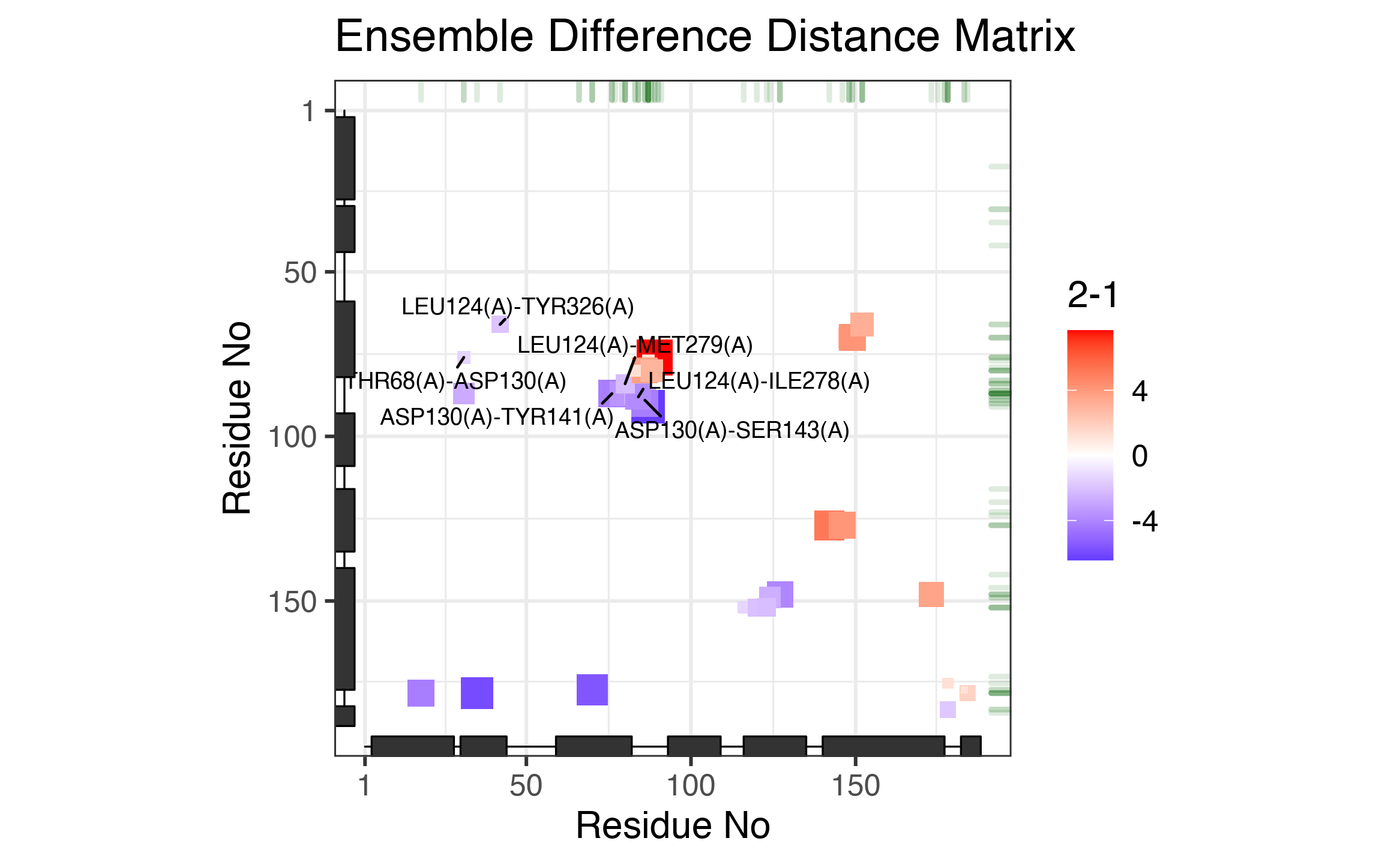
The ‘tile’ plot of identified significant distance changes. Each tile represents a residue pair with color and size scaled by the associated distance change from Group 1 to Group 2 (unit: angstrom).
Box-whisker plots of select pairs can also be generated for more specific comparisons.
# See Figure 5.
p <- boxplot(keys, dm, grps, inds = c(1:3,17:19))
p <- p + ggplot2::scale_color_manual(values=c("gray30", "#F8766D"), name="Group")
print(p)
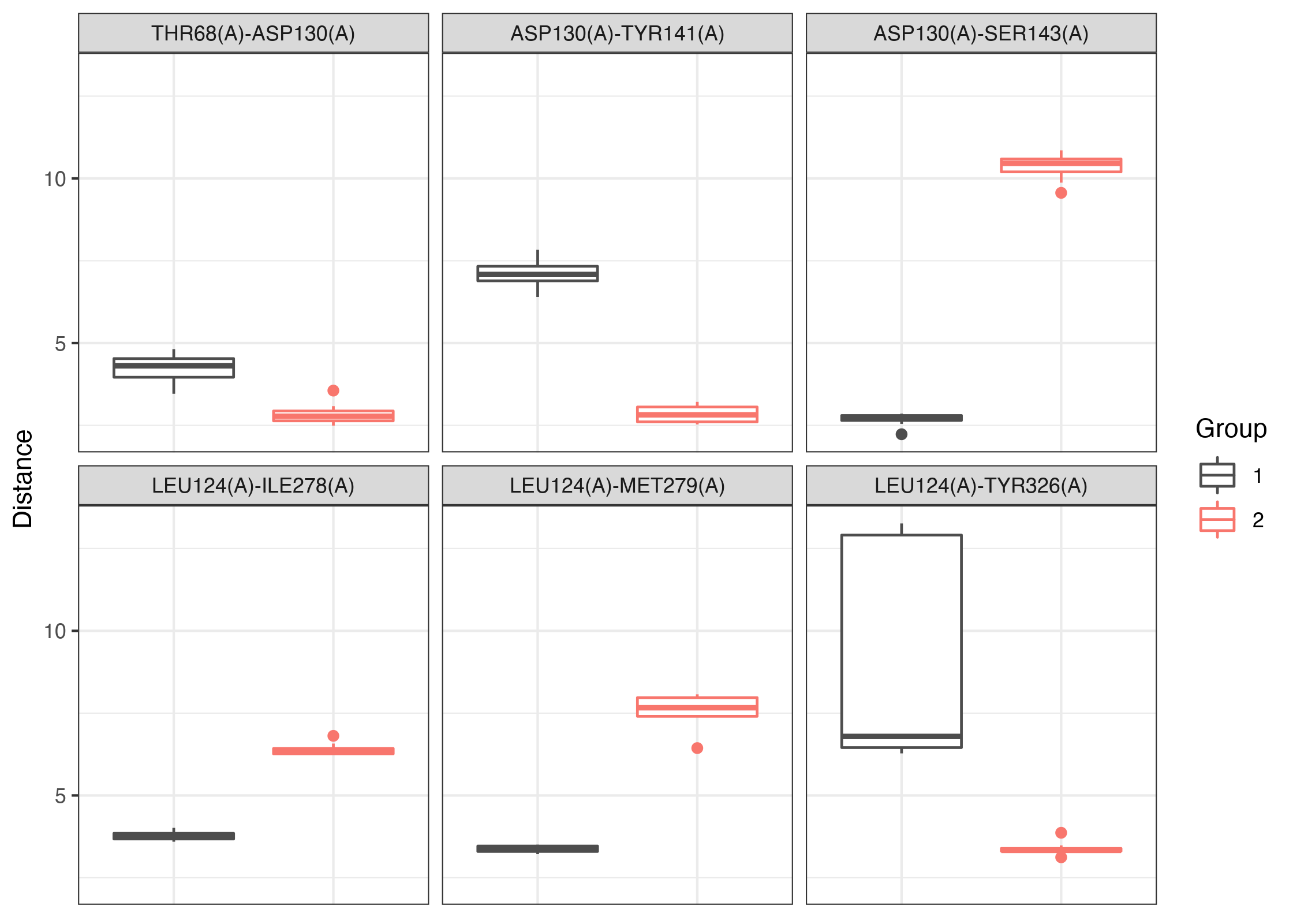
Box-whisker plots of select residue pairs.
Note that in the above, we use the scale_color_manual() function from the ggplot2 package to overide the default coloring scheme, in order to match the coloring in the PCA conformer plot (Figure 3).
Finally, 3D views of identified residue pairs mapped onto GPCR structures are generated. This is done by the pymol.eddm() (invoked by calling pymol()) Bio3D function. Before that, structural fitting is performed to facilitate the visual comparision.2
core <- core.find(pdbs)
Again, the following step is dependent on whether the pre-assembled or reconstructed dataset is used.
If using the pre-assembled “gpcr” dataset:
xyz <- pdbfit(pdbs, inds=core, outpath="fitlsq", prefix="pdbs/split_chain/",
              pdbext=".pdb")
Otherwise, if using the dataset constructed from scratch:
xyz <- pdbfit(pdbs, inds=core, outpath="fitlsq")
For convenience, we update the stored coordinates using the “fitted” structures.
pdbs$xyz <- xyz
We then view all identified key residue pairs showing significant distance changes using the pymol() Bio3D function. Note that the function generates a script file that needs to be opened by the PyMol software. In the following example, the key residues are displayed as “sticks”, through specifying as="sticks" in the function. See ?pymol.eddm for more types of representations.
# See Figures 6-8.
pymol(keys, pdbs=pdbs, grps=grps, as="sticks")
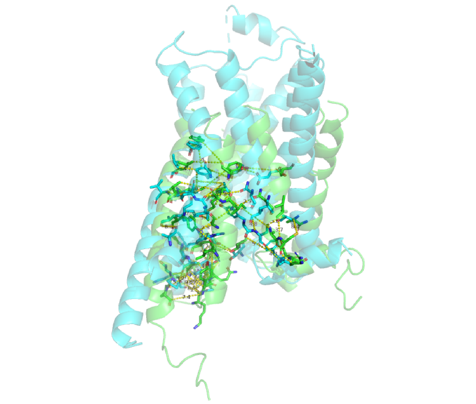
Use of pymol() to visualize all identified residue pairs (as sticks). Two GPCR structures are superimposed (green, inactive from PDB: 2R4R; cyan, active from PDB: 3SN6).
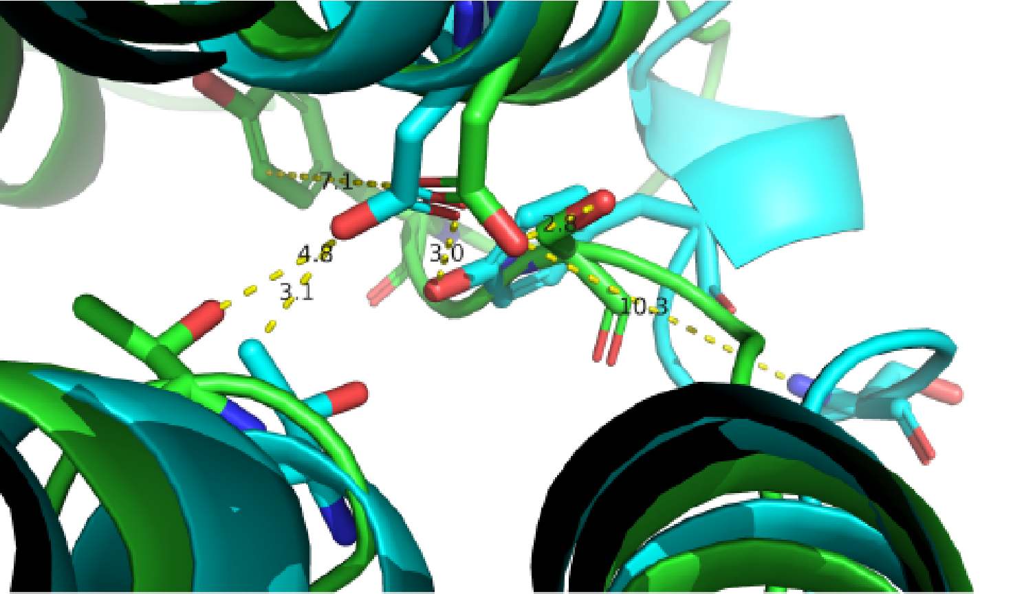
A close view of the switching region near ICL2. Two GPCR structures are superimposed (green, inactive from PDB: 2R4R; cyan, active from PDB: 3SN6).
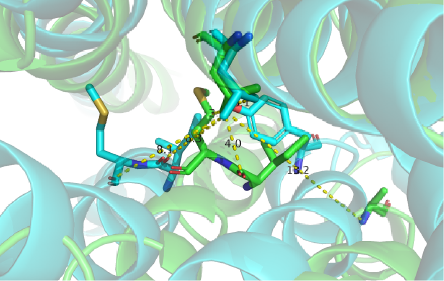
A close view of the switching region in the middle of TM helices. Two GPCR structures are superimposed (green, inactive from PDB: 2R4R; cyan, active from PDB: 3SN6).
detach(gpcr)
About this document
This document is generated by the rmarkdown R package. To reproduce it, simply type following commands:3
Information about the current Bio3D session
print(sessionInfo(), FALSE)
## R version 4.0.2 (2020-06-22)
## Platform: x86_64-apple-darwin17.0 (64-bit)
## Running under: macOS Catalina 10.15.6
##
## Matrix products: default
## BLAS:   /Library/Frameworks/R.framework/Versions/4.0/Resources/lib/libRblas.dylib
## LAPACK: /Library/Frameworks/R.framework/Versions/4.0/Resources/lib/libRlapack.dylib
##
## attached base packages:
## [1] stats     graphics  grDevices utils     datasets  methods   base
##
## other attached packages:
## [1] bio3d.eddm_0.1.0.9000 bio3d_2.4-1.9000
##
## loaded via a namespace (and not attached):
##  [1] Rcpp_1.0.5         cpp11_0.2.1        plyr_1.8.6         compiler_4.0.2
##  [5] pillar_1.4.6       highr_0.8          tools_4.0.2        digest_0.6.25
##  [9] evaluate_0.14      memoise_1.1.0      lifecycle_0.2.0    tibble_3.0.3
## [13] gtable_0.3.0       pkgconfig_2.0.3    rlang_0.4.7        ggrepel_0.8.2
## [17] yaml_2.2.1         parallel_4.0.2     pkgdown_1.6.1.9000 xfun_0.17
## [21] stringr_1.4.0      dplyr_1.0.2.9000   knitr_1.29         desc_1.2.0
## [25] generics_0.0.2     fs_1.5.0           vctrs_0.3.4        systemfonts_0.3.1
## [29] rprojroot_1.3-2    grid_4.0.2         tidyselect_1.1.0   glue_1.4.2
## [33] R6_2.4.1           rmarkdown_2.3      reshape2_1.4.4     farver_2.0.3
## [37] purrr_0.3.4        ggplot2_3.3.2      magrittr_1.5       backports_1.1.9
## [41] scales_1.1.1       htmltools_0.5.0    ellipsis_0.3.1     assertthat_0.2.1
## [45] colorspace_1.4-1   labeling_0.3       ragg_0.3.1         stringi_1.5.3
## [49] munsell_0.5.0      crayon_1.3.4
References
Grant, B. J., A. P. D. C Rodrigues, K. M. Elsawy, A. J. Mccammon, and L. S. D. Caves. 2006. “Bio3d: An R Package for the Comparative Analysis of Protein Structures.” Bioinformatics 22: 2695–6. https://doi.org/10.1093/bioinformatics/btl461.
Grant, B. J., L. Skjaerven, and X. Q. Yao. 2020. “The Bio3D Packages for Structural Bioinformatics.” Protein Sci in press. https://doi.org/DOI:10.1002/pro.3923.
Skjaerven, L., X. Q. Yao, G. Scarabelli, and B. J. Grant. 2014. “Integrating Protein Structural Dynamics and Evolutionary Analysis with Bio3d.” BMC Bioinformatics 15: 399. https://doi.org/10.1186/s12859-014-0399-6.