Comparative Protein Structure Analysis with Bio3D
Xin-Qiu Yao, Lars Skjaerven & Barry J. Grant
Bio3D_pca.RmdBackground
Bio3D1 is a group of R packages that provide interactive tools for the analysis of bimolecular structure, sequence and simulation data. The aim of this document, termed a vignette2 in R parlance, is to provide a brief task-oriented introduction to facilities for analyzing protein structure data with the Bio3D core package, bio3d (Grant et al. 2006).
Requirements
Detailed instructions for obtaining and installing the Bio3D packages on various platforms can be found in the Installing Bio3D vignette available online. Note that to follow along with this vignette the MUSCLE multiple sequence alignment program must be installed on your system and in the search path for executables. Please see the installation vignette for full details. This particular vignette was generated using bio3d version 2.4.1.9000.
Getting Started
Start R, load bio3d and use the command demo("pdb") and then demo("pca") to get a quick feel for some of the tasks that we will be introducing in the following sections.
Side-note:
You will be prompted to hit the RETURN key at each step of the demos as this will allow you to see the particular functions being called. Also note that detailed documentation and example code for each function can be accessed via the help() and example() commands (e.g. help(read.pdb)). You can also copy and paste any of the example code from the documentation of a particular function, or indeed this vignette, directly into your R session to see how things work. You can also find this documentation online.
Working with single PDB structures
A comprehensive introduction to working with PDB format structures with Bio3D can be found in PDB structure manipulation and analysis vignette. Here we confine ourselves to a very brief overview. The code snippet below calls the read.pdb() function with a single input argument, the four letter Protein Data Bank (PDB) identifier code "1tag". This will cause the read.pdb() function to read directly from the online RCSB PDB database and return a new object pdb for further manipulation.
pdb <- read.pdb("1tag")
## Note: Accessing on-line PDB fileAlternatively, you can read a PDB file directly from your local file system using the file name (or the full path to the file) as an argument to read.pdb():
A short summary of the pdb object can be obtained by calling the function print.pdb() (or simply typing pdb, which is equivalent in this case):
pdb
##
##  Call:  read.pdb(file = "1tag")
##
##    Total Models#: 1
##      Total Atoms#: 2890,  XYZs#: 8670  Chains#: 1  (values: A)
##
##      Protein Atoms#: 2521  (residues/Calpha atoms#: 314)
##      Nucleic acid Atoms#: 0  (residues/phosphate atoms#: 0)
##
##      Non-protein/nucleic Atoms#: 369  (residues: 342)
##      Non-protein/nucleic resid values: [ GDP (1), HOH (340), MG (1) ]
##
##    Protein sequence:
##       ARTVKLLLLGAGESGKSTIVKQMKIIHQDGYSLEECLEFIAIIYGNTLQSILAIVRAMTT
##       LNIQYGDSARQDDARKLMHMADTIEEGTMPKEMSDIIQRLWKDSGIQACFDRASEYQLND
##       SAGYYLSDLERLVTPGYVPTEQDVLRSRVKTTGIIETQFSFKDLNFRMFDVGGQRSERKK
##       WIHCFEGVTCIIFIAALSAYDMVLVEDDEVNRMHESLHLFNSICN...<cut>...DIII
##
## + attr: atom, xyz, seqres, helix, sheet,
##         calpha, remark, call
To examine the contents of the pdb object in more detail we can use the attributes function:
attributes(pdb)
## $names
## [1] "atom"   "xyz"    "seqres" "helix"  "sheet"  "calpha" "remark" "call"
##
## $class
## [1] "pdb" "sse"
These attributes describe the list components that comprise the pdb object, and each individual component can be accessed using the $ symbol (e.g. pdb$atom). Their complete description can be found on the read.pdb() functions help page accessible with the command: help(read.pdb). Note that the atom component is a data frame (matrix like object) consisting of all atomic coordinate ATOM/HETATM data, with a row per ATOM and a column per record type. The column names can be used as a convenient means of data access, for example to access coordinate data for the first three atoms in our newly created pdb object:
pdb$atom[1:3, c("resno","resid","elety","x","y","z")]
##   resno resid elety      x      y      z
## 1    27   ALA     N 38.238 18.018 61.225
## 2    27   ALA    CA 38.552 16.715 60.576
## 3    27   ALA     C 40.042 16.687 60.253
In the example above we used numeric indices to access atoms 1 to 3, and a character vector of column names to access the specific record types. In a similar fashion the atom.select() function returns numeric indices that can be used for accessing desired subsets of the pdb data. For example:
ca.inds <- atom.select(pdb, "calpha")
The returned ca.inds object is a list containing atom and xyz numeric indices corresponding to the selection (all C-alpha atoms in this particular case). The indices can be used to access e.g. the Cartesian coordinates of the selected atoms (pdb$xyz[, ca.inds$xyz]), or residue numbers and B-factor data for the selected atoms. For example:
# See Figure 1
bf <- pdb$atom$b[ca.inds$atom]
plot.bio3d(bf, resno=pdb, sse=pdb, ylab="B-factor", xlab="Residue", typ="l")
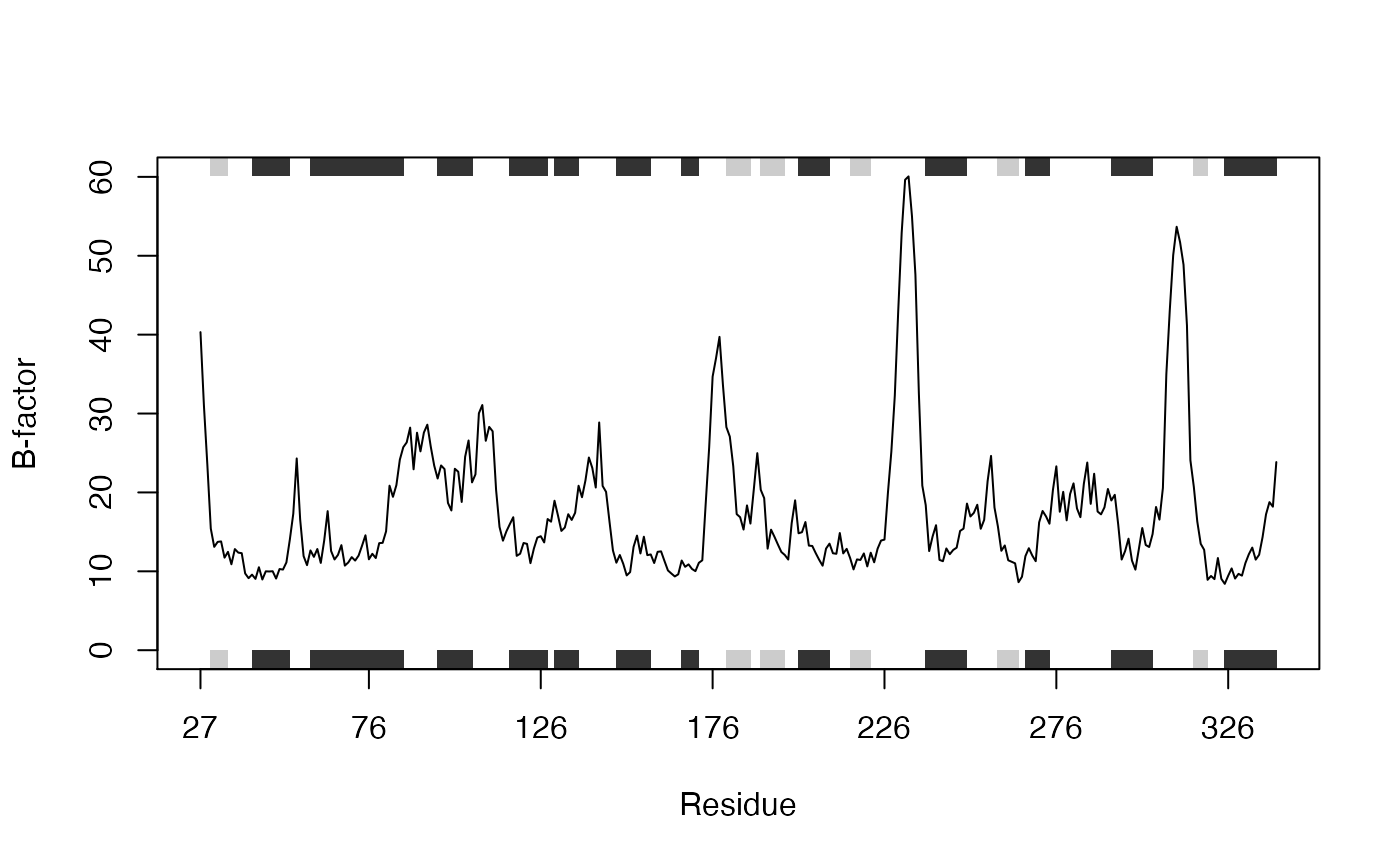
Residue B-factor data for PDB id 1TAG. Grey boxes depict secondary structure elements in the structure (dark grey: alpha helices; light grey: beta sheets).
In the above example we use these indices to plot residue number (taken from the pdb object, note these residue numbers do not start at 1) vs B-factor along with a basic secondary structure schematic (again taken from the pdb object and provided with the argument sse=pdb; Figure 1). Note also that we could access this same data with pdb$atom[ca.inds$atom, "b"]. As a further example of data access lets extract the sequence for the loop region (P-loop) between beta 1 (the third strand in the beta sheet) and alpha 1 in our pdb object.
loop <- pdb$sheet$end[3]:pdb$helix$start[1]
loop.inds <- atom.select(pdb, resno=loop, elety="CA")
pdb$atom[loop.inds$atom, "resid"]
## [1] "LEU" "GLY" "ALA" "GLY" "GLU" "SER" "GLY" "LYS"In the above example the residue numbers in the sheet and helix components of pdb are accessed and used in a subsequent atom selection, the output of which is used as indices to extract residue names.
Since Bio3D version 2.1 the component in the PDB object is in a matrix format (as compared to a vector format in previous versions). Thus, notice the extra comma in the square bracket operator when accessing Cartesian coordinates from the object ().
Question:
How would you extract the one-letter amino acid sequence for the loop region mentioned above? HINT: The aa321() function converts between three-letter and one-letter IUPAC amino acid codes.
Question:
How would you select all backbone or sidechain atoms? HINT: see the example section of help(atom.select) and the string option.
Side-note:
Consider the combine.select function for combining multiple atom selections. See help(combine.select) and additional vignettes for more details.
Note that if you know a particular sequence pattern or motif characteristic of a region of interest you could access it via a sequence search as follows:
aa <- pdbseq(pdb)
aa[ motif.find(".G....GK[ST]", aa )]
##  35  36  37  38  39  40  41  42  43
## "L" "G" "A" "G" "E" "S" "G" "K" "S"
Working with multiple PDB structures
The Bio3D package was designed to specifically facilitate the analysis of multiple structures from both experiment and simulation. The challenge of working with these structures is that they are usually different in their composition (i.e. contain differing number of atoms, sequences, chains, ligands, structures, conformations etc. even for the same protein as we will see below) and it is these differences that are frequently of most interest.
For this reason Bio3D contains extensive utilities to enable the reading and writing of sequence and structure data, sequence and structure alignment, performing homologous protein searches, structure annotation, atom selection, re-orientation, superposition, rigid core identification, clustering, torsion analysis, distance matrix analysis, structure and sequence conservation analysis, normal mode analysis across related structures, and principal component analysis of structural ensembles. We will demonstrate some of these utilities in the following sections. More comprehensive demonstrations for special tasks, e.g. various operations of PDB structures, analysis of MD trajectories and normal mode analysis can be found in corresponding vignettes.
Before delving into more advanced analysis lets examine how we can read multiple PDB structures from the RCSB PDB for a particular protein and perform some basic analysis:
# Download some example PDB files
ids <- c("1TND_B","1AGR_A","1FQJ_A","1TAG_A","1GG2_A","1KJY_A")
raw.files <- get.pdb(ids)
The get.pdb() function will download the requested files, below we extract the particular chains we are most interested in with the function pdbsplit() (note these ids could come from the results of a blast.pdb() search as described in subsequent sections). The requested chains are then aligned and their structural data stored in a new object pdbs that can be used for further analysis and manipulation.
# Extract and align the chains we are interested in
files <- pdbsplit(raw.files, ids)
pdbs <- pdbaln(files)
Below we examine their sequence and structural similarity.
# Calculate sequence identity
pdbs$id <- substr(basename(pdbs$id),1,6)
seqidentity(pdbs)
##        1TND_B 1AGR_A 1FQJ_A 1TAG_A 1GG2_A 1KJY_A
## 1TND_B  1.000  0.693  0.914  1.000  0.690  0.696
## 1AGR_A  0.693  1.000  0.779  0.694  0.997  0.994
## 1FQJ_A  0.914  0.779  1.000  0.914  0.776  0.782
## 1TAG_A  1.000  0.694  0.914  1.000  0.691  0.697
## 1GG2_A  0.690  0.997  0.776  0.691  1.000  0.991
## 1KJY_A  0.696  0.994  0.782  0.697  0.991  1.000
## Calculate RMSD rmsd(pdbs, fit=TRUE)
##        1TND_B 1AGR_A 1FQJ_A 1TAG_A 1GG2_A 1KJY_A
## 1TND_B  0.000  0.965  0.609  1.283  1.612  2.100
## 1AGR_A  0.965  0.000  0.873  1.575  1.777  1.914
## 1FQJ_A  0.609  0.873  0.000  1.265  1.737  2.042
## 1TAG_A  1.283  1.575  1.265  0.000  1.687  1.841
## 1GG2_A  1.612  1.777  1.737  1.687  0.000  1.879
## 1KJY_A  2.100  1.914  2.042  1.841  1.879  0.000
Question:
What effect does setting the fit=TRUE option have in the RMSD calculation? What would the results indicate if you set fit=FALSE or disparaged this option? HINT: Bio3D functions have various default options that will be used if the option is not explicitly specified by the user, see help(rmsd) for an example and note that the input options with an equals sign (e.g. fit=FALSE) have default values.
Exploring example data for the transducin heterotrimeric G Protein
A number of example datasets are included with the Bio3D core package. The main purpose of including this data (which may be generated by the user by following the extended examples documented within the various Bio3D functions) is to allow users to more quickly appreciate the capabilities of functions that would otherwise require extensive data downloads before execution.
For a number of the examples in the current vignette we will utilize the included transducin dataset that contains over 50 publicly available structures. This dataset formed the basis of the work described in (Yao and Grant 2013) and we refer the motivated reader to this publication and references therein for extensive background information. Briefly, heterotrimeric G proteins are molecular switches that turn on and off intracellular signaling cascades in response to the activation of G protein coupled receptors (GPCRs). Receptor activation by extracellular stimuli promotes a cycle of GTP binding and hydrolysis on the G protein alpha subunit that leads to conformational rearrangements (i.e. internal structural changes) that activate multiple downstream effectors. The current dataset consists of transducin (including Gt and Gi/o) alpha subunit sequence and structural data and can be accessed with the command attach(transducin):
attach(transducin)
Side-note:
This dataset can be assembled from scratch with commands similar to those detailed in the next section and those listed in section 2.2. Also see help(example.data) for a full description of this dataset’s contents.
Constructing Experimental Structure Ensembles for a Protein Family
Comparing multiple structures of homologous proteins and carefully analyzing large multiple sequence alignments can help identify patterns of sequence and structural conservation and highlight conserved interactions that are crucial for protein stability and function (Grant et al. 2007). Bio3D provides a useful framework for such studies and can facilitate the integration of sequence, structure and dynamics data in the analysis of protein evolution.
Finding Available Sets of Similar Structures
In this tutorial, to collect available transducin crystal structures, we first use BLAST to query the PDB database to find similar sequences (and hence structures) to our chosen representative (PDB Id: 1TAG):
Examining the alignment scores and their associated E-values (with the function plot.blast()) indicates a sensible normalized score (-log(E-Value)) cutoff of 240 bits (Figure 2).
# See Figure 2.
hits <- plot.blast(blast, cutoff=240)
##   * Possible cutoff values:    242 6
##             Yielding Nhits:    66 106
##
##   * Chosen cutoff value of:    240
##             Yielding Nhits:    66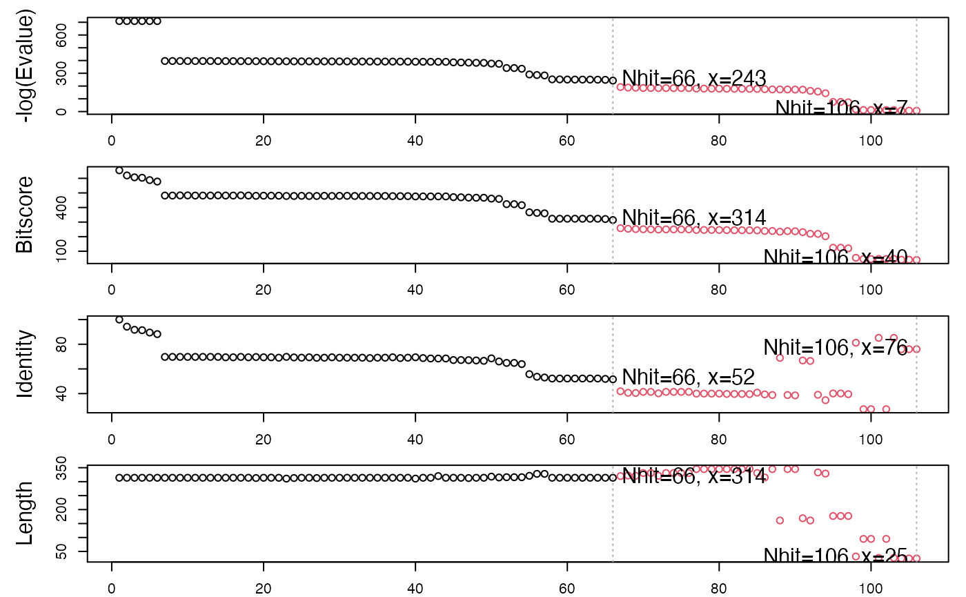
Summary of BLAST results for query 1tag against the PDB chain database
We can then list a subset of our top hits, for example:
head(hits$hits)
##   pdb.id   acc      group
## 1 "1TAD_A" "1TAD_A" "1"
## 2 "6OY9_A" "6OY9_A" "1"
## 3 "3V00_A" "3V00_A" "1"
## 4 "1FQJ_A" "1FQJ_A" "1"
## 5 "6OYA_A" "6OYA_A" "1"
## 6 "1GOT_A" "1GOT_A" "1"head(hits$pdb.id)
## [1] "1TAD_A" "6OY9_A" "3V00_A" "1FQJ_A" "6OYA_A" "1GOT_A"Sidenote:
The function pdb.annotate() can fetch detailed information about the corresponding structures (e.g. title, experimental method, resolution, ligand name(s), citation, etc.). For example:
anno <- pdb.annotate(hits)
head(anno[, c("resolution", "ligandId", "citation")])
##        resolution       ligandId                         citation
## 1TAD_A        1.7 ALF,CA,CAC,GDP      Sondek et al. Nature (1994)
## 6OY9_A        3.9           <NA>       Gao et al. Mol.Cell (2019)
## 3V00_A        2.9            GDP Singh et al. Biochemistry (2012)
## 1FQJ_A       2.02     ALF,GDP,MG        Slep et al. Nature (2001)
## 6OYA_A        3.3           <NA>       Gao et al. Mol.Cell (2019)
## 1GOT_A        2.0            MSE   Lambright et al. Nature (1996)
Multiple Sequence Alignment
Next we download the complete list of structures from the PDB (with function get.pdb()), and use function pdbsplit() to split the structures into separate chains and store them for subsequent access. Finally, function pdbaln() will extract the sequence of each structure and perform a multiple sequence alignment to determine residue-residue correspondences (NOTE: requires external program MUSCLE be in search path for executables):
# Download PDBs and split by chain ID
files <- get.pdb(hits, path="raw_pdbs", split = TRUE)

# Extract and align sequences
pdbs <- pdbaln(files)
You can now inspect the alignment (the automatically generated “aln.fa” file) with your favorite alignment viewer (we recommend SEAVIEW, available from: http://pbil.univ-lyon1.fr/software/seaview.html).
Side-note:
You may find a number of structures with missing residues (i.e. gaps in the alignment) at sites of particular interest to you. If this is the case you may consider removing these structures from your hit list and generating a smaller, but potentially higher quality, dataset for further exploration.
Question:
How could you automatically identify gap positions in your alignment? HINT: try the command help.search("gap", package="bio3d").
Comparative Structure Analysis
The detailed comparison of homologous protein structures can be used to infer pathways for evolutionary adaptation and, at closer evolutionary distances, mechanisms for conformational change. Bio3D employs both conventional methods for structural analysis (alignment, RMSD, difference distance matrix analysis, etc.) as well as refined structural superposition and principal component analysis (PCA) to facilitate comparative structure analysis.
Structure Superposition
Conventional structural superposition of proteins minimizes the root mean square difference between their full set of equivalent residues. This can be performed with Bio3D functions pdbfit() and fit.xyz() as outlined previously. However, for certain applications such a superposition procedure can be inappropriate. For example, in the comparison of a multi-domain protein that has undergone a hinge-like rearrangement of its domains, standard all atom superposition would result in an underestimate of the true atomic displacement by attempting superposition over all domains (whole structure superposition). A more appropriate and insightful superposition would be anchored at the most invariant region and hence more clearly highlight the domain rearrangement (sub-structure superposition).
The Bio3D core.find() function implements an iterated superposition procedure, where residues displaying the largest positional differences are identified and excluded at each round. The function returns an ordered list of excluded residues, from which the user can select a subset of ’core’ residues upon which superposition can be based.
core <- core.find(pdbs)
The plot.core() and print.core() functions allow one to further examine the output of the core.find() procedure (see below and Figure 3).
# See Figure 3.
col=rep("black", length(core$volume))
col[core$volume<2]="pink"; col[core$volume<1]="red"
plot(core, col=col)
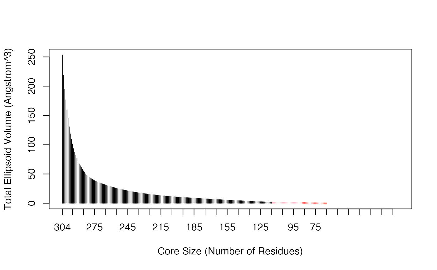
Identification of core residues
The print.core() function also returns atom and xyz indices similar to those returned from the atom.select() function. Below we use these indices for core superposition and to write a quick PDB file for viewing in a molecular graphics program such as VMD (Figure 4).
core.inds <- print(core, vol=1.0)
## # 88 positions (cumulative volume <= 1 Angstrom^3)
##    start end length
## 1     32  52     21
## 2    195 195      1
## 3    216 226     11
## 4    239 239      1
## 5    242 247      6
## 6    260 274     15
## 7    279 279      1
## 8    282 283      2
## 9    295 304     10
## 10 317 336 20write.pdb(xyz=pdbs$xyz[1,core.inds$xyz], file="quick_core.pdb")
The most structural invariant core positions in the transducin family
We can now superpose all structures on the selected core indices with the fit.xyz() or pdbfit() function.
xyz <- pdbfit( pdbs, core.inds )
The above command performs the actual superposition and stores the new coordinates in the matrix object xyz.
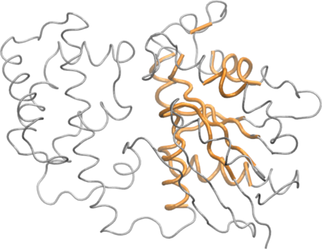
Side-note:
By providing an extra outpath="somedir" argument to pdbfit the superposed structures can be output for viewing (in this case to the local directory somedir which you can obviously change). These fitted structures can then be viewed in your favorite molecular graphics program (Figure 5).
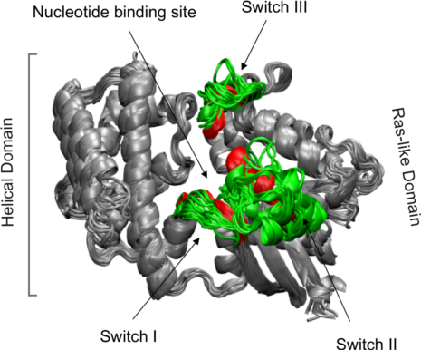
Structure ensemble of transducin family superposed based on core positions
Standard Structural Analysis
Bio3D contains functions to perform standard structural analysis, such as root mean-square deviation (RMSD), root mean-square fluctuation (RMSF), secondary structure, dihedral angles, difference distance matrices etc. The current section provides a brief exposure to using Bio3D in this vein. However, do feel free to skip ahead to the arguably more interesting section on PCA analysis.
Root mean square deviation (RMSD):
RMSD is a standard measure of structural distance between coordinate sets. Here we examine the pairwise RMSD values and cluster our structures based on these values:
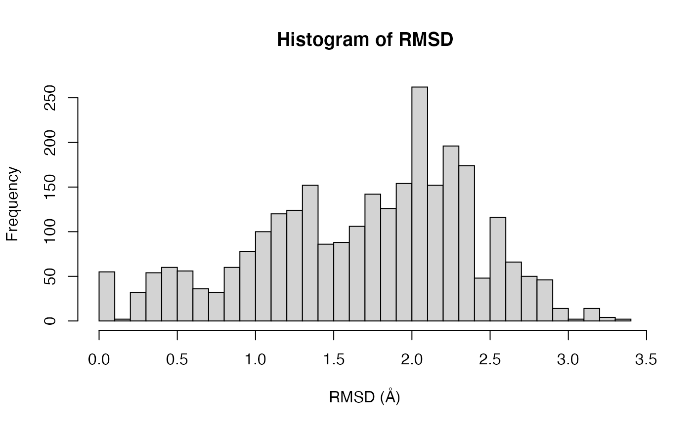
Histogram of RMSD among transducin structures
The result can be illustrated as a simple dendrogram with the command:
pdbs$id <- substr(basename(pdbs$id), 1, 6)
hclustplot(hc.rd, colors=annotation[, "color"], labels=pdbs$id, cex=0.5,
          ylab="RMSD (Å)", main="RMSD Cluster Dendrogram", fillbox=FALSE)
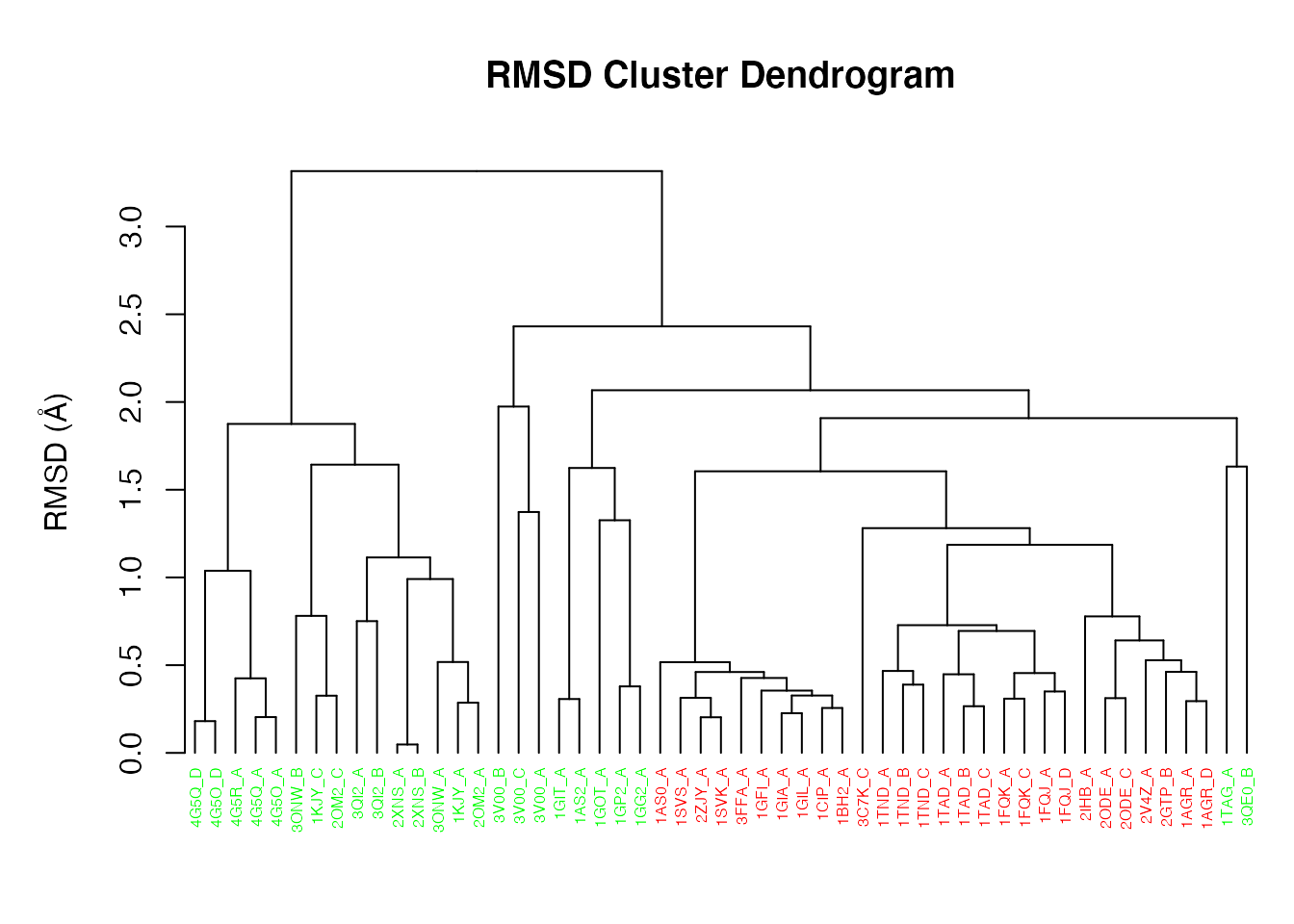
RMSD clustering of transducin structures
Question:
How many structure groups/clusters do we have according to this clustering? How would determine which structures are assigned to which cluster? HINT: See help(cutree).
Question:
What kind of plot would the command heatmap(rd) produce? How would you label this plot with PDB codes? HINT: labCol and labRow.
Root mean squared fluctuations (RMSF):
RMSF is another often used measure of conformational variance. The Bio3D rmsf() function returns a vector of atom-wise (or residue-wise) variance instead of a single numeric value. The below sequence of commands returns the indices for gap containing positions, which we then exclude from subsequent RMSF calculation:
# Ignore gap containing positions
gaps.res <- gap.inspect(pdbs$ali)
gaps.pos <- gap.inspect(pdbs$xyz)

# Tailor the PDB structure to exclude gap positions for SSE annotation
id <- grep("1TAG", pdbs$id)
inds <- atom.select(pdb, resno = pdbs$resno[id, gaps.res$f.inds])
ref.pdb <- trim.pdb(pdb, inds = inds)

# Plot RMSF with SSE annotation and labeled with residue numbers (Figure 8.)
rf <- rmsf(xyz[, gaps.pos$f.inds])
plot.bio3d(rf, resno=ref.pdb, sse=ref.pdb, ylab="RMSF (Å)",
           xlab="Residue No.", typ="l")
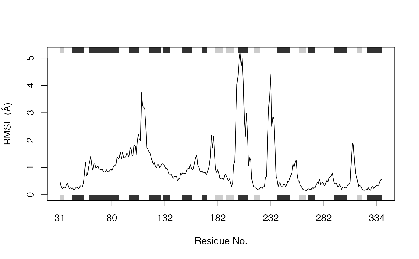
RMSF plot
Torsion/Dihedral analysis:
The conformation of a polypeptide or nucleotide chain can be usefully described in terms of angles of internal rotation around its constituent bonds.
tor <- torsion.pdb(pdb)

# Basic Ramachandran plot (Figure 9)
plot(tor$phi, tor$psi, xlab="phi", ylab="psi")

Basic Ramachandran plot
Lets compare the Calpha atom based pseudo-torsion angles between two structures, the inactive (PDB Id: 1TAG) and active (PDB Id: 1TND) transducin alpha subunit:
# Locate the two structures in pdbs
ind.a <- grep("1TAG_A", pdbs$id)
ind.b <- grep("1TND_B", pdbs$id)

# Exclude gaps in the two structures to make them comparable
gaps.xyz2 <- gap.inspect(pdbs$xyz[c(ind.a, ind.b), ])
a.xyz <- pdbs$xyz[ind.a, gaps.xyz2$f.inds]
b.xyz <- pdbs$xyz[ind.b, gaps.xyz2$f.inds]

# Compare CA based pseudo-torsion angles between the two structures
a <- torsion.xyz(a.xyz, atm.inc=1)
b <- torsion.xyz(b.xyz, atm.inc=1)
d.ab <- wrap.tor(a-b)
d.ab[is.na(d.ab)] <- 0

# Plot results with SSE annotation
plot.bio3d(abs(d.ab), resno=pdb, sse=pdb, typ="h", xlab="Residue No.",
           ylab = "Difference Angle")
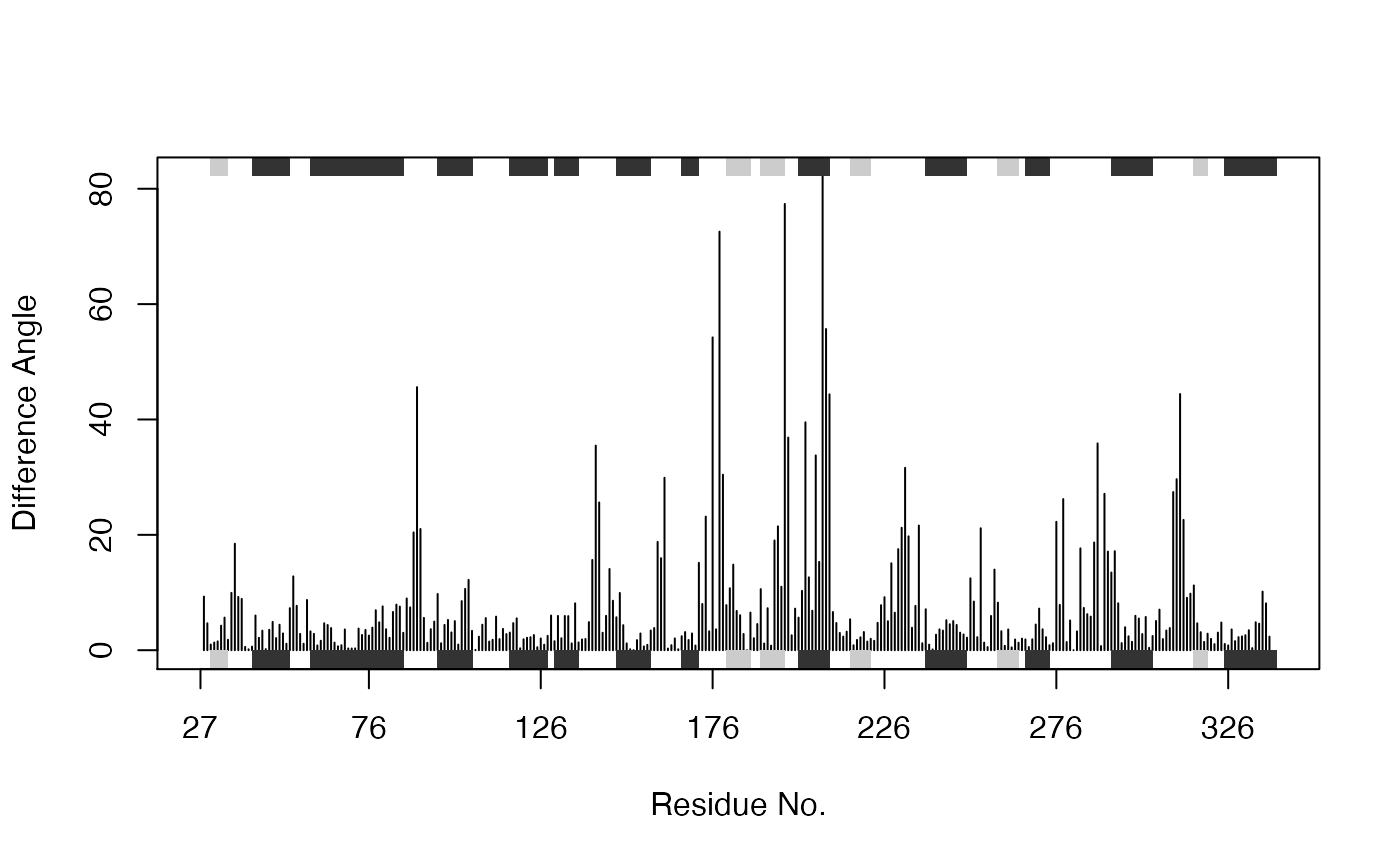
Torsion angle difference between structures in inactive GDP bound (1tag) and active GTP analogue bound (1tnd) states
Difference distance matrix analysis (DDM)
Distance matrices can be calculated with the function dm() and contact maps with the function cmap(). In the example below we calculate the difference distance matrix by simply subtracting one distance matrix from another. Note the vectorized nature of the this calculation (i.e. we do not have to explicitly iterate through each element of the matrix):
a <- dm.xyz(a.xyz)
b <- dm.xyz(b.xyz)

plot.dmat( (a - b), nlevels=10, grid.col="gray", xlab="1tag", ylab="1tnd")
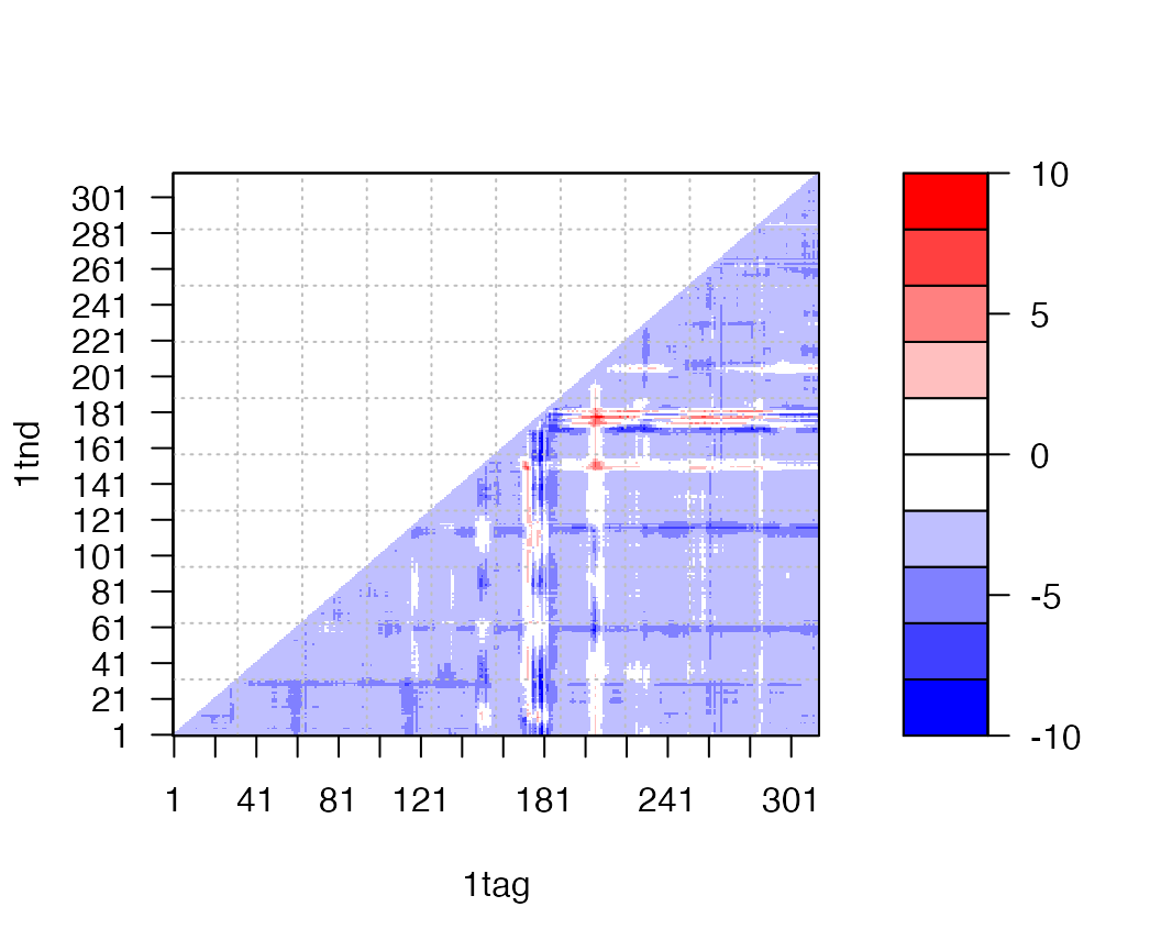
Difference of distance matrices between structures in GDP(1tag) and GTP(1tnd) nucleotide states
Principal Component Analysis (PCA)
Following core identification and subsequent superposition, PCA can be employed to examine the relationship between different structures based on their equivalent residues. The application of PCA to both distributions of experimental structures and molecular dynamics trajectories, along with its ability to provide considerable insight into the nature of conformational differences is also discussed in the molecular dynamics trajectory analysis vignette.
Briefly, the resulting principal components (orthogonal eigenvectors) describe the axes of maximal variance of the distribution of structures. Projection of the distribution onto the space defined by the largest principal components results in a lower dimensional representation of the structural dataset. The percentage of the total mean square displacement (or variance) of atom positional fluctuations captured in each dimension is characterized by their corresponding eigenvalue. Experience suggests that 3–5 dimensions are often sufficient to capture over 70 percent of the total variance in a given family of structures. Thus, a handful of principal components are sufficient to provide a useful description while still retaining most of the variance in the original distribution (Grant et al. 2006).
The below command excludes the gap positions identified above from the PCA (note you can also simply run pca(xyz, rm.gaps=TRUE)).
# Do PCA
pc.xray <- pca.xyz(xyz[, gaps.pos$f.inds])
pc.xray
##
## Call:
##   pca.xyz(xyz = xyz[, gaps.pos$f.inds])
##
## Class:
##   pca
##
## Number of eigenvalues:
##   915
##
##         Eigenvalue Variance Cumulative
##    PC 1    259.521   49.794     49.794
##    PC 2     81.302   15.599     65.393
##    PC 3     40.095    7.693     73.086
##    PC 4     29.701    5.699     78.785
##    PC 5     24.048    4.614     83.399
##    PC 6     19.611    3.763     87.162
##
##    (Obtained from 53 conformers with 915 xyz input values).
##
## + attr: L, U, z, au, sdev, mean, call
Question:
Why is the input to function pca.xyz() given as xyz rather than pdbs$xyz?
Question:
Why would you need superposition before using pca.xyz but not need it for pca.tor?
A quick overview of the results of pca.xyz() can be obtained by calling print.pca() and plot.pca() (Figure 12).
plot(pc.xray, col=annotation[, "color"])
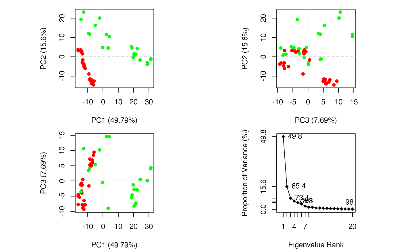
Overview of PCA results for transducin crystallographic structures
Setting the option pc.axes will allow for single plots to also be produced in this way, e.g.:
plot(pc.xray, pc.axes=1:2, col=annotation[, "color"])
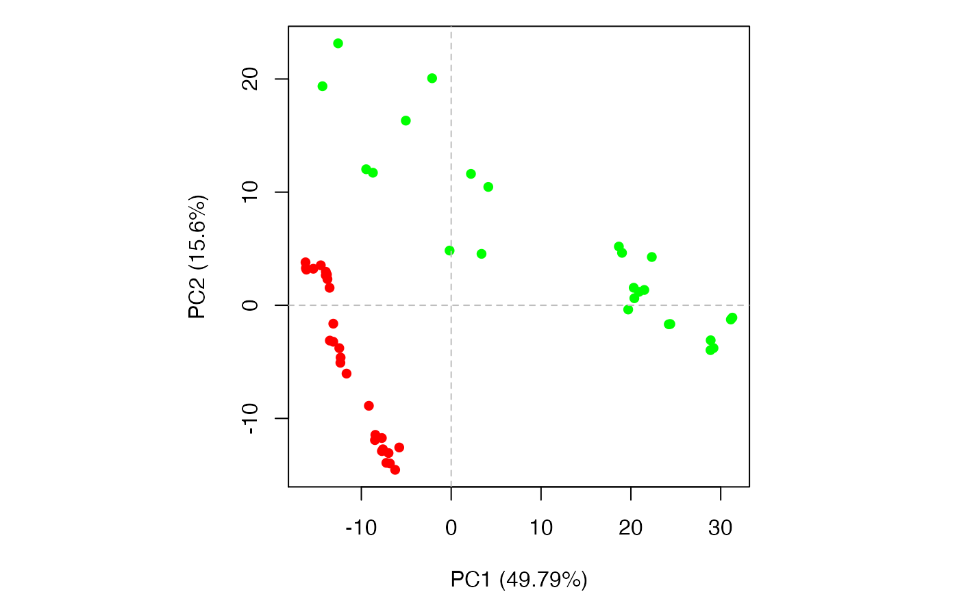
Results of setting pc.axes=1:2 in plot.pca() function
One can then use the identify() function to label and individual points.
# Left-click on a point to label and right-click to end
identify(pc.xray$z[,1:2], labels=basename.pdb(pdbs$id))
We can also call plot.bio3d() to examine the contribution of each residue to the first three principal components with the following commands (Figure 13).
par(mfrow = c(3, 1), cex = 0.75, mar = c(3, 4, 1, 1))
plot.bio3d(pc.xray$au[,1], resno=ref.pdb, sse=ref.pdb, ylab="PC1")
plot.bio3d(pc.xray$au[,2], resno=ref.pdb, sse=ref.pdb, ylab="PC2")
plot.bio3d(pc.xray$au[,3], resno=ref.pdb, sse=ref.pdb, ylab="PC3")
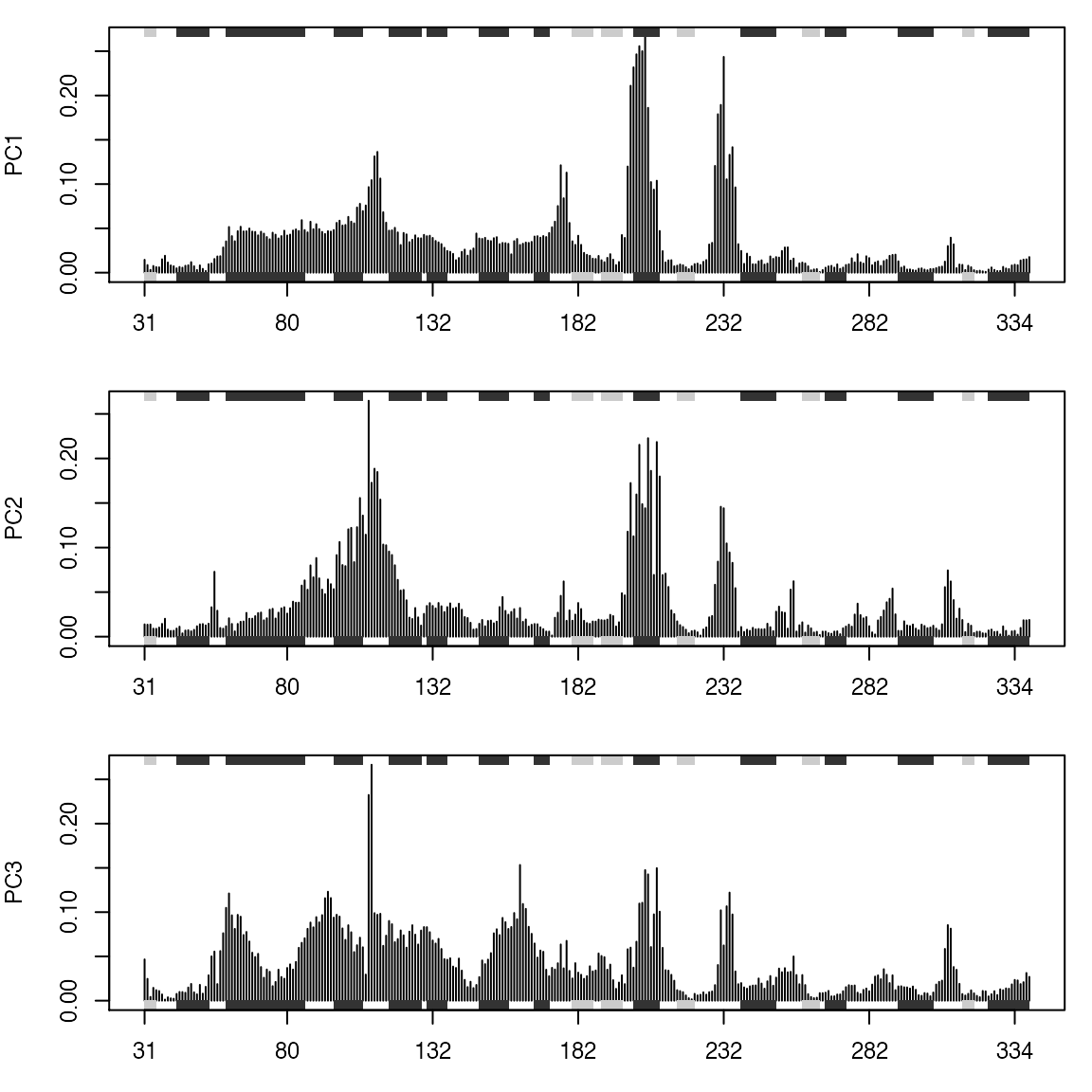
Contribution of each residue to the first three principal components
The plots in Figures 12-14 display the relationships between different conformers, highlight positions responsible for the major differences between structures and enable the interpretation and characterization of multiple interconformer relationships.
To further aid interpretation, a PDB format trajectory can be produced that interpolates between the most dissimilar structures in the distribution along a given principal component. This involves dividing the difference between the conformers into a number of evenly spaced steps along the principal components, forming the frames of the trajectory. Such trajectories can be directly visualized in a molecular graphics program, such as VMD (Humphrey 1996) (Figure 15). Furthermore, the PCA results can be compared to those from simulations (see the molecular dynamics and normal mode analysis vignettes), as well as guiding dynamic network analysis, being analyzed for possible dynamic domains (with the Bio3D geostas() function from the bio3d.geostas package), domain and shear movements with the DynDom package (Hayward and Berendsen 1998), or used as initial seed structures for reaction path refinement methods such as Conjugate Peak Refinement (Fischer and Karplus 1992).
# See Figure 15
mktrj.pca(pc.xray, pc=1, file="pc1.pdb")
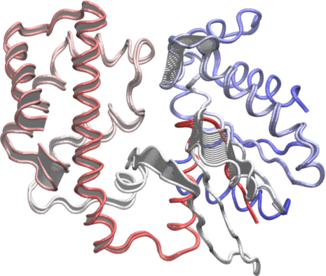
Interpolated structures along PC1 produced by the mktrj.pca() function
Conformer Clustering in PC Space
Clustering structures in PC space can often enable one to focus on the relationships between individual structures in terms of their major structural displacements, with a controllable level of dynamic details (via specifying the number of PCs used in the clustering). For example, with clustering along PCs 1 and 2, we can investigate how the X-ray structures of transducin relate to each other with respect to the major conformation change that covers over 65% of their structural variance (See Figures 12). This can reveal functional relationships that are often hard to find by conventional pairwise methods such as the RMSD clustering detailed previously (Figure 7). For example in the PC1-PC2 plane, the inactive “GDP” structures (green points in Figure 12) are further split into two sub-groups (Figures 16 and 17). The bottom-right sub-group (blue) exclusively correspond to the structures complexed with GDP dissociation inhibitor (GDI). This functionaly distinct state is clearly evident in the PC plot and clustering dendrogram that can be generated with the following commands:
hc <- hclust(dist(pc.xray$z[,1:2]))
grps <- cutree(hc, h=30)
cols <- c("red", "green", "blue")[grps]
plot(pc.xray, pc.axes=1:2, col=cols)
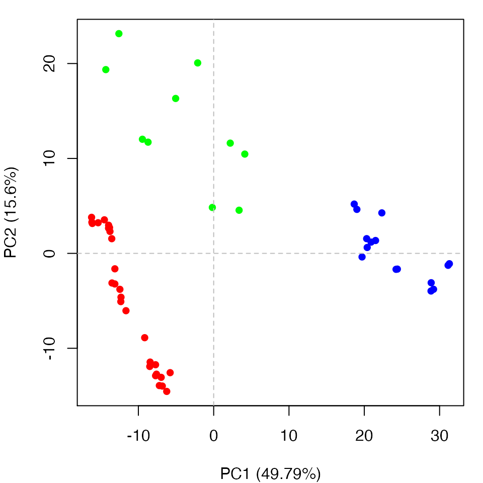
Clustering based on PC1-PC2. Note the new blue cluster are all GDI bound forms (see text for details)
# Dendrogram plot
names(cols) <- pdbs$id
hclustplot(hc, colors=cols, ylab="Distance in PC Space", main="PC1-2", cex=0.5)
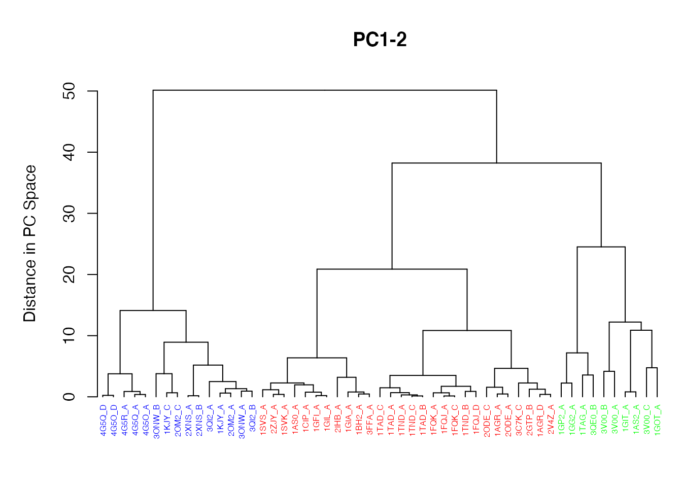
Clustering based on PC1-PC2
Sidenote:
On the PC1 vs PC2 conformer plot in Figure 16 you can interactively identify and label individual structures by using the identify() function clicking with your mouse (left to select, right to end). In this particular case the command would be:
identify(pc.xray$z[,1], pc.xray$z[,2], labels=pdbs$id)
Where to Next
If you have read this far, congratulations! We are ready to have some fun and move to other package vignettes that describe more interesting analysis including Correlation Network Analysis (where we will build and dissect dynamic networks form different correlated motion data), enhanced methods for Normal Mode Analysis (where we will explore the dynamics of large protein families and superfamilies using predictive calculations), and advanced Comparative Structure Analysis (where we will mine available experimental data and supplement it with simulation results to map the conformational dynamics and coupled motions of proteins).
Document Details
This document is available from the Bio3D website in R markdown, PDF, and HTML formats. All code can be extracted and automatically executed to generate Figures and/or the PDF with the following commands:
Information About the Current Bio3D Session
## R version 4.0.2 (2020-06-22)
## Platform: x86_64-apple-darwin17.0 (64-bit)
## Running under: macOS Catalina 10.15.6
##
## Matrix products: default
## BLAS:   /Library/Frameworks/R.framework/Versions/4.0/Resources/lib/libRblas.dylib
## LAPACK: /Library/Frameworks/R.framework/Versions/4.0/Resources/lib/libRlapack.dylib
##
## locale:
## [1] en_US.UTF-8/en_US.UTF-8/en_US.UTF-8/C/en_US.UTF-8/en_US.UTF-8
##
## attached base packages:
## [1] stats     graphics  grDevices utils     datasets  methods   base
##
## other attached packages:
## [1] bio3d_2.4-1.9000
##
## loaded via a namespace (and not attached):
##  [1] Rcpp_1.0.5         cpp11_0.2.1        knitr_1.29         magrittr_1.5
##  [5] R6_2.4.1           ragg_0.3.1         rlang_0.4.7        stringr_1.4.0
##  [9] highr_0.8          tools_4.0.2        parallel_4.0.2     grid_4.0.2
## [13] xfun_0.17          htmltools_0.5.0    systemfonts_0.3.1  yaml_2.2.1
## [17] assertthat_0.2.1   rprojroot_1.3-2    digest_0.6.25      pkgdown_1.6.1.9000
## [21] crayon_1.3.4       bitops_1.0-6       fs_1.5.0           RCurl_1.98-1.2
## [25] memoise_1.1.0      evaluate_0.14      rmarkdown_2.3      stringi_1.5.3
## [29] compiler_4.0.2     desc_1.2.0         backports_1.1.9    XML_3.99-0.5
References
Fischer, S., and M. Karplus. 1992. “Conjugate Peak Refinement: An Algorithm for Finding Reaction Paths and Accurate Transition States in Systems with Many Degrees of Freedom.” Chem. Phys. Lett 194: 252–61.
Grant, B. J., A. J. Mccammon, L. S. D. Caves, and R. A. Cross. 2007. “Multivariate Analysis of Conserved Sequence-Structure Relationships in Kinesins: Coupling of the Active Site and a Tubulin-Binding Sub-Domain.” J. Mol. Biol 5: 1231–48.
Grant, B. J., A. P. D. C Rodrigues, K. M. Elsawy, A. J. Mccammon, and L. S. D. Caves. 2006. “Bio3d: An R Package for the Comparative Analysis of Protein Structures.” Bioinformatics 22: 2695–6.
Hayward, S., and H. Berendsen. 1998. “Systematic Analysis of Domain Motions in Proteins from Conformational Change: New Results on Citrate Synthase and T4 Lysozyme.” Proteins 30: 144–54.
Humphrey, et al., W. 1996. “VMD: Visual Molecular Dynamics.” J. Mol. Graph 14: 33–38.
Yao, X. Q., and B. J. Grant. 2013. “Domain-Opening and Dynamic Coupling in the Alpha-Subunit of Heterotrimeric G Proteins.” Biophys. J 105: L08–10.
The latest version of the package, full documentation and further vignettes (including detailed installation instructions) can be obtained from the main Bio3D website: http://thegrantlab.org/bio3d/↩︎
This vignette contains executable examples, see
help(vignette)for further details.↩︎