Ensemble NMA of E.coli DHFR structures
Lars Skjaerven, Xin-Qiu Yao, Guido Scarabelli & Barry J. Grant
Bio3D_nma-dhfr-partI.RmdBackground
Bio3D1 is an R package that provides interactive tools for structural bioinformatics. The primary focus of Bio3D is the analysis of bimolecular structure, sequence and simulation data (Grant et al. 2006).
Normal mode analysis (NMA) is one of the major simulation techniques used to probe large-scale motions in biomolecules. Typical application is for the prediction of functional motions in proteins. Version 2.0 of the Bio3D package now includes extensive NMA facilities (Skjaerven et al. 2015). These include a unique collection of multiple elastic network model force-fields, automated ensemble analysis methods, and variance weighted NMA (see also the NMA Vignette). Here we provide an in-depth demonstration of ensemble NMA with working code that comprise complete executable examples2.
Requirements
Detailed instructions for obtaining and installing the Bio3D package on various platforms can be found in the Installing Bio3D Vignette available both on-line and from within the Bio3D package. In addition to Bio3D the MUSCLE multiple sequence alignment program (available from the muscle home page must be installed on your system and in the search path for executables. Please see the installation vignette for further details.
Part I: Ensemble NMA of E.coli DHFR structures
In this vignette we perform ensemble NMA on the complete collection of E.coli Dihydrofolate reductase (DHFR) structures in the protein data-bank (PDB). Starting from only one PDB identifier (PDB ID 1rx2) we show how to search the PDB for related structures using BLAST, fetch and align the structures, and finally calculate the normal modes of each individual structure in order to probe for potential differences in structural flexibility.
Search and retrieve DHFR structures
Below we perform a blast search of the PDB database to identify related structures to our query E.coli DHFR sequence. In this particular example we use function get.seq() to fetch the query sequence for chain A of the PDB ID 1RX2 and use this as input to blast.pdb(). Note that get.seq() would also allow the corresponding UniProt identifier.
## Registered S3 methods overwritten by 'bio3d.nma':
##   method     from
##   dccm.egnm  bio3d
##   dccm.enma  bio3d
##   dccm.gnm   bio3d
##   dccm.nma   bio3d
##   mktrj.enma bio3d
##   mktrj.nma  bio3d
##   plot.enma  bio3d
##   plot.nma   bio3d
##   plot.rmsip bio3d
##   print.enma bio3d
##   print.nma  bio3d
##   pymol.nma  bio3d
##
## Attaching package: 'bio3d.nma'## The following objects are masked from 'package:bio3d':
##
## aanma, bhattacharyya, build.hessian, cov.enma, cov.nma,
## covsoverlap, difference.vector, ff.aaenm, ff.aaenm2, ff.anm,
## ff.calpha, ff.pfanm, ff.reach, ff.sdenm, fluct.nma, gnm,
## load.enmff, nma, overlap, rmsip, rtb, sip, var.pdbs, var.xyzaa <- get.seq("1rx2_A")
## Fetching... Please wait. Done.blast <- hmmer(aa, verbose=FALSE)
Function plot.blast() facilitates the visualization and filtering of the Blast results. It will attempt to set a seed position to the point of largest drop-off in normalized scores (i.e. the biggest jump in E-values). In this particular case we specify a cutoff (after initial plotting) of 225 to include only the relevant E.coli structures:
hits <- plot(blast, cutoff=232)
##   * Possible cutoff values:    241 2
##             Yielding Nhits:    144 766
##
##   * Chosen cutoff value of:    232
##             Yielding Nhits:    144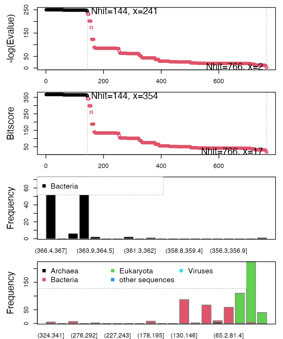
Blast results. Visualize and filter blast results through function plot.blast(). Here we proceed with only the top scoring hits (black).
The Blast search and subsequent filtering identified a total of 101 related PDB structures to our query sequence. The PDB identifiers of this collection are accessible through the pdb.id attribute to the hits object (hits$pdb.id). Note that adjusting the cutoff argument (to plot.blast()) will result in a decrease or increase of hits.
We can now use function get.pdb() and pdbslit() to fetch and parse the identified structures. Finally, we use pdbaln() to align the PDB structures.
# fetch PDBs
raw.files <- get.pdb(hits$pdb.id, path = "raw_pdbs", gzip=TRUE)
# split by chain ID
files <- pdbsplit(raw.files, ids = hits$pdb.id, path = "raw_pdbs/split_chain", ncore=4)
# align structures
pdbs.all <- pdbaln(files, fit=TRUE)
The pdbs.all object now contains aligned C-alpha atom data, including Cartesian coordinates, residue numbers, residue types, and B-factors. The sequence alignment is also stored by default to the FASTA format file ‘aln.fa’ (to view this you can use an alignment viewer such as SEAVIEW, see Requirements section above). In cases where manual edits of the alignment are necessary you can re-read the sequence alignment and coordinate data with:
aln <- read.fasta('aln.fa')
pdbs.all <- read.fasta.pdb(aln)
At this point the pdbs.all object contains all identified 101 structures. This might include structures with missing residues, and/or multiple structurally redundant conformers. For our subsequent NMA missing in-structure residues might bias the calculation, and redundant structures can be useful to omit to reduce the computational load. Below we inspect the connectivity of the PDB structures with a function call to inspect.connectivity(), and trim.pdbs() to filter out those structures from our pdbs.all object. Similarly, we omit structures that are conformationally redundant to reduce the computational load with function filter.rmsd():
# remove structures with missing residues
conn <- inspect.connectivity(pdbs.all, cut=4.05)
pdbs <- trim(pdbs.all, row.inds=which(conn))

# which structures are omitted
which(!conn)

# remove conformational redundant structures
rd <- filter.rmsd(pdbs$xyz, cutoff=0.1, fit=TRUE)
pdbs <- trim(pdbs, row.inds=rd$ind)

# remove "humanized" e-coli dhfr
excl <- unlist(lapply(c("3QL0", "4GH8"), grep, toupper(pdbs$id)))
pdbs <- trim(pdbs, row.inds=which(!(1:length(pdbs$id) %in% excl)))

# a list of PDB codes of our final selection
ids <- unlist(strsplit(basename(pdbs$id), split=".pdb"))
Use print() to see a short summary of the pdbs object:
print(pdbs, alignment=FALSE)
##
## Call:
##   trim.pdbs(pdbs = pdbs, row.inds = which(!(1:length(pdbs$id) %in%
##     excl)))
##
## Class:
##   pdbs, fasta
##
## Alignment dimensions:
##   121 sequence rows; 166 position columns (159 non-gap, 7 gap)
##
## + attr: id, xyz, resno, b, chain, ali, resid, call
Annotate collected PDB structures
Function pdb.annotate() provides a convenient way of annotating the PDB files we have collected. Below we use the function to annotate each structure to its source species. This will come in handy when annotating plots later on:
anno <- pdb.annotate(ids)
print(unique(anno$source))
## [1] "Escherichia coli"Principal component analysis
A principal component analysis (PCA) can be performed on the structural ensemble (stored in the pdbs object) with function pca.xyz(). To obtain meaningful results we first superimpose all structures on the invariant core (function core.find()).
# find invariant core
core <- core.find(pdbs)

# superimpose all structures to core
pdbs$xyz = pdbfit(pdbs, core$c0.5A.xyz)

# identify gaps, and perform PCA
gaps.pos <- gap.inspect(pdbs$xyz)
gaps.res <- gap.inspect(pdbs$ali)
pc.xray <- pca.xyz(pdbs$xyz[,gaps.pos$f.inds])
# plot PCA
plot(pc.xray)
Note that a call to the wrapper function pca() would provide identical results as the above code:
pc.xray <- pca(pdbs, core.find=TRUE)
Function rmsd() will calculate all pairwise RMSD values of the structural ensemble. This facilitates clustering analysis based on the pairwise structural deviation:
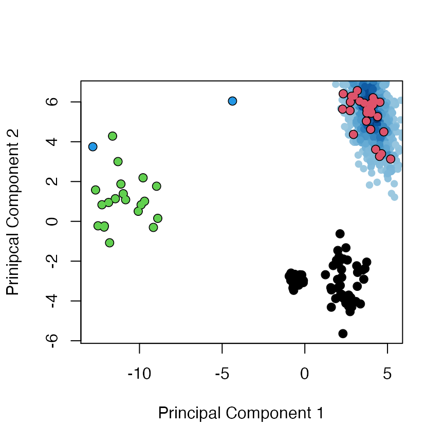
plot(pc.xray$z[,1:2], col="grey50", pch=16, cex=1.3,
     ylab="Prinipcal Component 2", xlab="Principal Component 1")
points(pc.xray$z[,1:2], col=grps.rd, pch=16, cex=0.9)
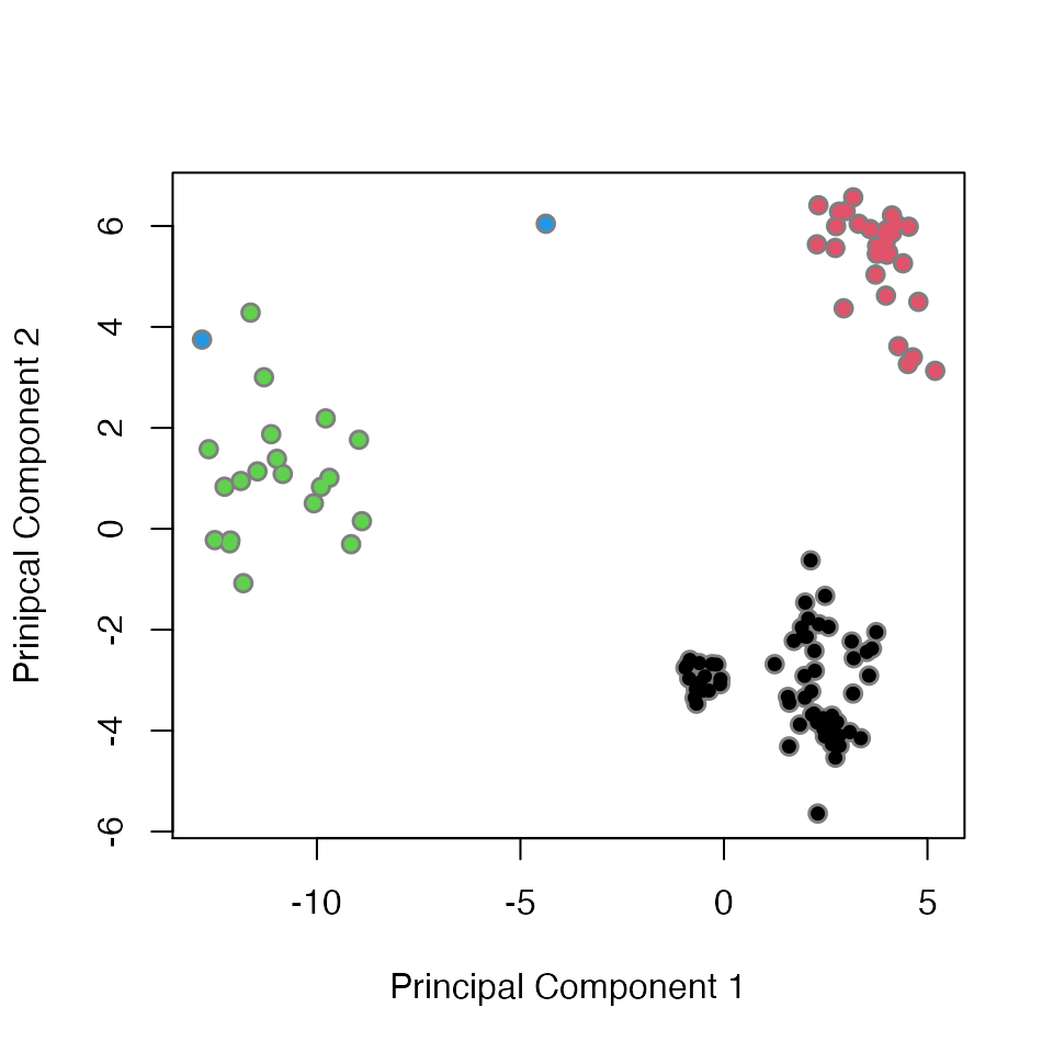
Projection of the X-ray conformers shows that the E.coli DHFR structures can be divided into three major groups along their two first eigenvectors: closed, open, and occluded conformations. Each dot is colored according to their cluster membership: occluded conformations (green), open conformations (black), and closed conformations (red).
To visualize the major structural variations in the ensemble function mktrj() can be used to generate a trajectory PDB file by interpolating along the eigenvector:
mktrj(pc.xray, pc=1,
      resno=pdbs$resno[1, gaps.res$f.inds],
      resid=pdbs$resid[1, gaps.res$f.inds])
Function pdbfit() can be used to write the PDB files to separate directories according to their cluster membership:
Normal modes analysis
Function nma.pdbs() will calculate the normal modes of each protein structure stored in the pdbs object. The normal modes are calculated on the full structures as provided by object pdbs. With the default argument rm.gaps=TRUE unaligned atoms are omitted from output:
modes <- nma(pdbs, rm.gaps=TRUE, ncore=4)
The modes object of class enma contains aligned normal mode data including fluctuations, RMSIP data, and aligned eigenvectors. A short summary of the modes object can be obtain by calling the function print(), and the aligned fluctuations can be plotted with function plot.enma().
print(modes)
##
## Call:
##   nma.pdbs(pdbs = pdbs, rm.gaps = TRUE, ncore = 4)
##
## Class:
##   enma
##
## Number of structures:
##   121
##
## Attributes stored:
##   - Root mean square inner product (RMSIP)
##   - Aligned atomic fluctuations
##   - Aligned eigenvectors (gaps removed)
##   - Dimensions of x$U.subspace: 477x471x121
##
## Coordinates were aligned prior to NMA calculations
##
## + attr: fluctuations, rmsip, U.subspace, L, full.nma, xyz,
##         call
# plot modes fluctuations plot(modes, pdbs=pdbs, col=grps.rd, label=NULL)
## Re-reading PDB (2inq_B) to extract SSE## /usr/local/bin/mkdssp## Warning in dssp.pdb(pdb.ref, ...): Non-protein residues detected in input PDB:
## MT1, HOH, DOD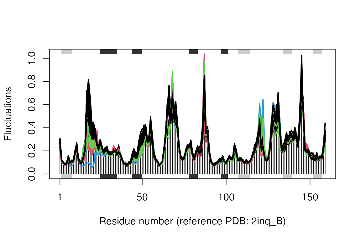
Normal mode fluctuations of the E.coli DHFR ensemble. Each line represent the mode fluctuations for the individual structures. Color coding according to structural clustering: green (occluded), black (open), and red (closed).
heatmap(1-modes$rmsip, distfun = as.dist, labRow = ids, labCol = ids,
        ColSideColors=as.character(grps.nma), RowSideColors=as.character(grps.rd))
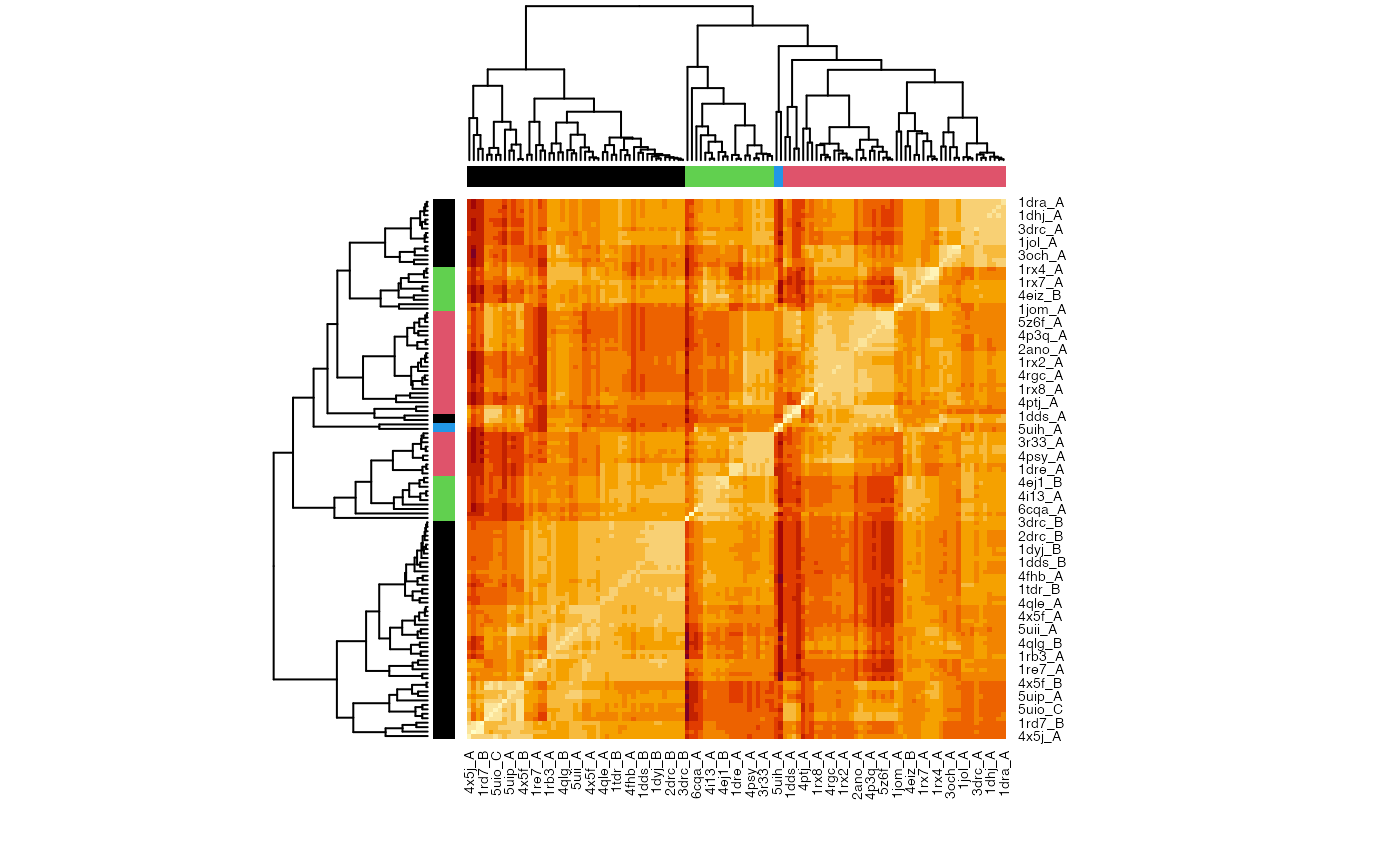
Clustering of structures based on their normal modes similarity (in terms of pair-wise RMSIP values).
Fluctuation analysis
Comparing the mode fluctuations of two groups of structures can reveal specific regions of distinct flexibility patterns. Below we focus on the differences between the open (black), closed (red) and occluded (green) conformations of the E.coli structures:
## Re-reading PDB (2inq_B) to extract SSE## /usr/local/bin/mkdssp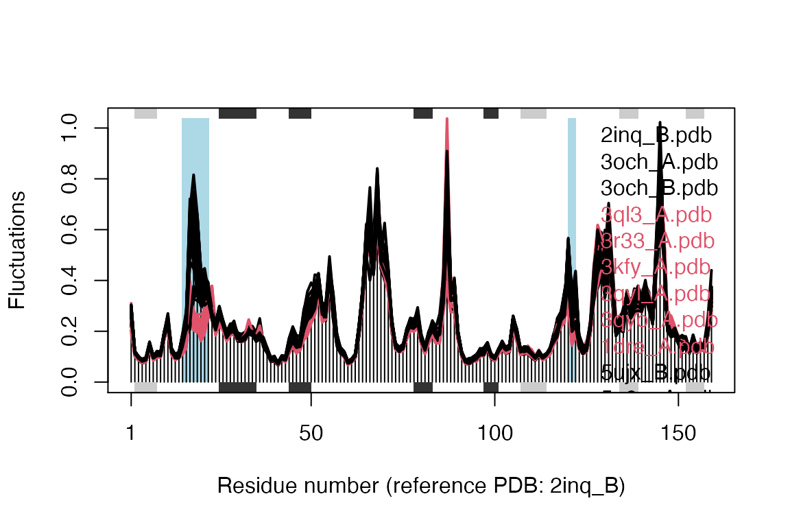
Comparison of mode fluctuations between open (black) and closed (red) conformers. Significant differences among the mode fluctuations between the two groups are marked with shaded blue regions.
## Re-reading PDB (2inq_B) to extract SSE## /usr/local/bin/mkdssp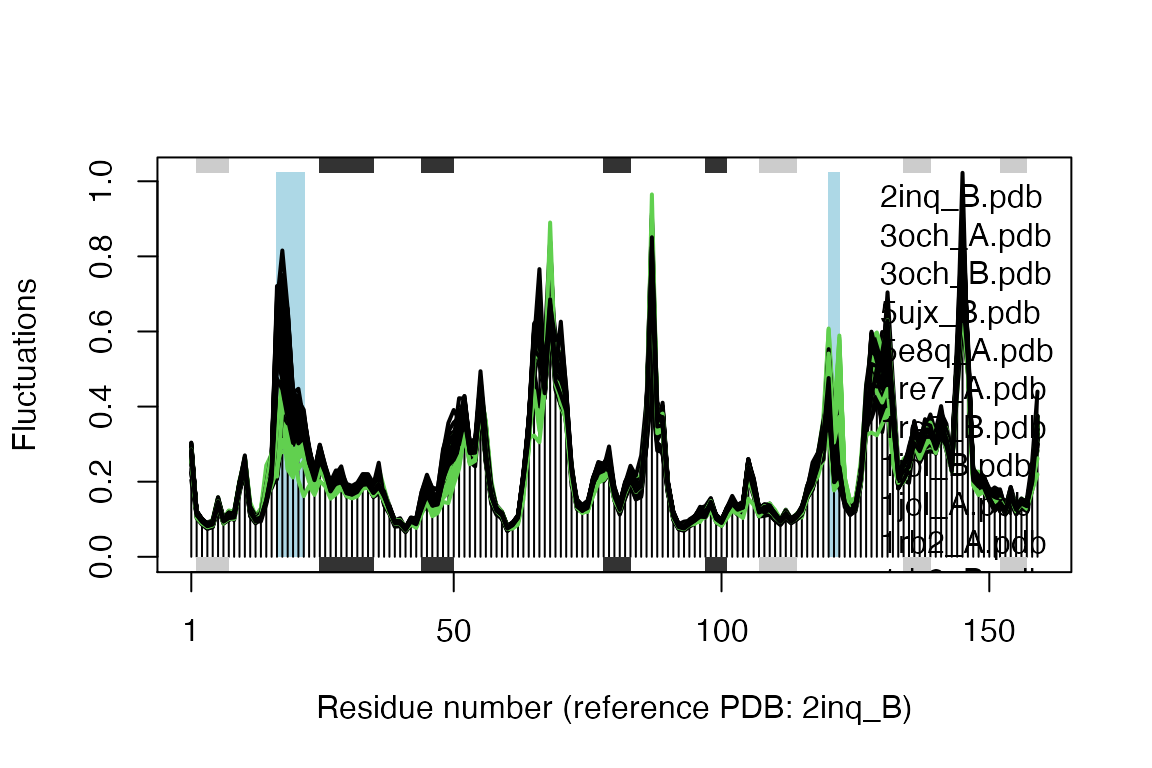
Comparison of mode fluctuations between open (black) and occluded (green) conformers. Significant differences among the mode fluctuations between the two groups are marked with shaded blue regions.
cols <- grps.rd
cols[which(grps.rd!=2 & grps.rd!=3)]=NA
plot(modes, pdbs=pdbs, col=cols, signif=TRUE)
## Re-reading PDB (3ql3_A) to extract SSE## PDB has ALT records, taking A only, rm.alt=TRUE## /usr/local/bin/mkdssp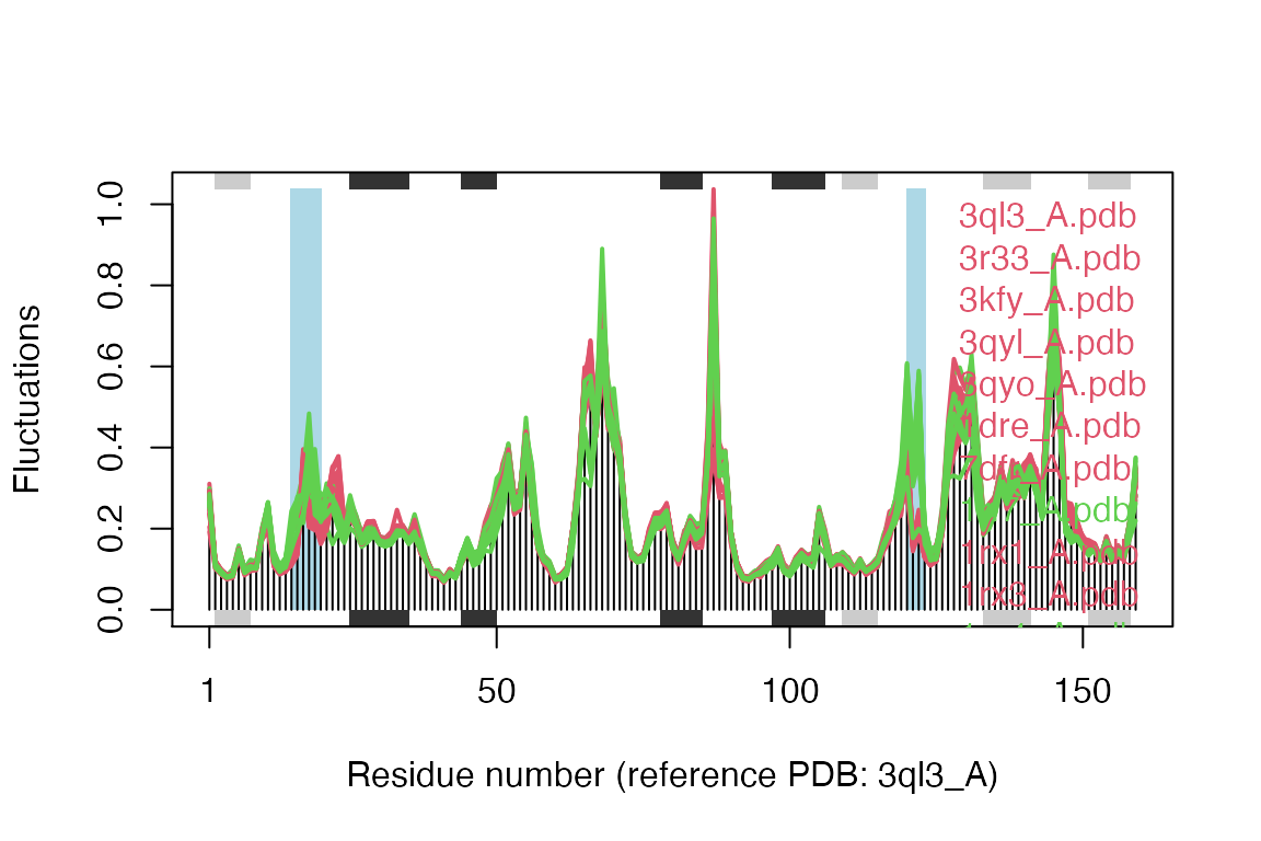
Comparison of mode fluctuations between closed (red) and occluded (green) conformers. Significant differences among the mode fluctuations between the two groups are marked with shaded blue regions.
Compare with MD simulation
The above analysis can also nicely be integrated with molecular dynamics (MD) simulations. Below we read in a 5 ns long MD trajectory (of PDB ID 1RX2). We visualize the conformational sampling by projecting the MD conformers onto the principal components (PCs) of the X-ray ensemble, and finally compare the PCs of the MD simulation to the normal modes:
pdb <- read.pdb("md-traj/1rx2-CA.pdb")
trj <- read.ncdf("md-traj/1rx2_5ns.nc")

inds <- pdb2aln.ind(pdbs, pdb, gaps.res$f.inds)
inds.core <- pdb2aln.ind(pdbs, pdb, core$c0.5A.atom)

# inds$a is for the pdbs object
# inds$b is for the MD structure

trj.fit <- fit.xyz(pdbs$xyz[1,], trj, core$c0.5A.xyz, inds.core$b$xyz)
proj <- project.pca(trj.fit[, inds$b$xyz], pc.xray)
cols <- densCols(proj[,1:2])
plot(proj[,1:2], col=cols, pch=16,
     ylab="Prinipcal Component 2", xlab="Principal Component 1",
     xlim=range(pc.xray$z[,1]), ylim=range(pc.xray$z[,2]))
points(pc.xray$z[,1:2], col=1, pch=1, cex=1.1)
points(pc.xray$z[,1:2], col=grps.rd, pch=16)
Projection of MD conformers onto the X-ray PC space provides a two dimensional representation of the conformational sampling along the MD simulation (blue dots).
# PCA of the MD trajectory
pc.md <- pca.xyz(trj.fit[, inds$b$xyz])

# compare MD-PCA and NMA
r <- rmsip(pc.md$U, modes$U.subspace[,,1])

print(r)
## $overlap
##        b1    b2    b3    b4    b5    b6    b7    b8    b9   b10
## a1  0.273 0.007 0.042 0.042 0.050 0.001 0.004 0.000 0.002 0.005
## a2  0.202 0.225 0.007 0.006 0.031 0.026 0.006 0.008 0.002 0.001
## a3  0.102 0.002 0.013 0.005 0.000 0.009 0.001 0.016 0.002 0.128
## a4  0.004 0.090 0.033 0.276 0.016 0.079 0.045 0.006 0.008 0.001
## a5  0.018 0.016 0.017 0.010 0.014 0.037 0.005 0.000 0.047 0.008
## a6  0.043 0.019 0.022 0.078 0.042 0.028 0.067 0.057 0.028 0.019
## a7  0.002 0.036 0.170 0.002 0.002 0.046 0.003 0.140 0.001 0.000
## a8  0.042 0.430 0.062 0.128 0.005 0.034 0.009 0.000 0.007 0.002
## a9  0.015 0.000 0.001 0.021 0.147 0.005 0.059 0.002 0.017 0.069
## a10 0.004 0.007 0.155 0.007 0.049 0.000 0.034 0.004 0.009 0.008
##
## $rmsip
## [1] 0.6390165
##
## attr(,"class")
## [1] "rmsip"plot(r, xlab="MD PCA", ylab="NMA")
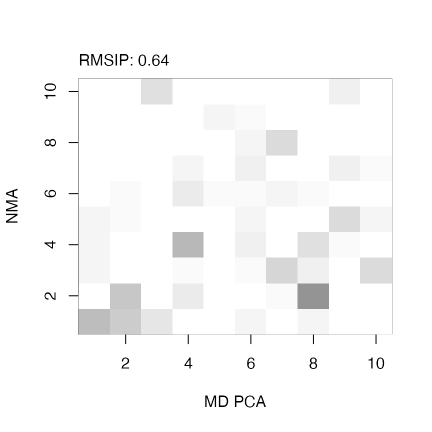
Overlap map between normal modes and principal components of a 5 ns long MD simulation. The two subsets yields an RMSIP value of 0.64, where a value of 1 would idicate identical directionality.
# compare MD-PCA and X-rayPCA
r <- rmsip(pc.md, pc.xray)
Domain analysis with GeoStaS
Identification of regions in the protein that move as rigid bodies is facilitated with the implementation of the GeoStaS algorithm (Romanowska, Nowinski, and Trylska 2012). Below we demonstrate the use of function geostas() on data obtained from ensemble NMA, an ensemble of PDB structures, and a 5 ns long MD simulation. See help(geostas) for more details and further examples.
library(bio3d.geostas)
## Warning: replacing previous import 'bio3d::overlap' by 'bio3d.nma::overlap' when
## loading 'bio3d.geostas'
## Warning: replacing previous import 'bio3d::cov.enma' by 'bio3d.nma::cov.enma'
## when loading 'bio3d.geostas'## Warning: replacing previous import 'bio3d::ff.calpha' by 'bio3d.nma::ff.calpha'
## when loading 'bio3d.geostas'## Warning: replacing previous import 'bio3d::ff.aaenm2' by 'bio3d.nma::ff.aaenm2'
## when loading 'bio3d.geostas'## Warning: replacing previous import 'bio3d::load.enmff' by
## 'bio3d.nma::load.enmff' when loading 'bio3d.geostas'## Warning: replacing previous import 'bio3d::covsoverlap' by
## 'bio3d.nma::covsoverlap' when loading 'bio3d.geostas'## Warning: replacing previous import 'bio3d::bhattacharyya' by
## 'bio3d.nma::bhattacharyya' when loading 'bio3d.geostas'## Warning: replacing previous import 'bio3d::nma' by 'bio3d.nma::nma' when loading
## 'bio3d.geostas'## Warning: replacing previous import 'bio3d::rmsip' by 'bio3d.nma::rmsip' when
## loading 'bio3d.geostas'## Warning: replacing previous import 'bio3d::ff.aaenm' by 'bio3d.nma::ff.aaenm'
## when loading 'bio3d.geostas'## Warning: replacing previous import 'bio3d::cov.nma' by 'bio3d.nma::cov.nma' when
## loading 'bio3d.geostas'## Warning: replacing previous import 'bio3d::aanma' by 'bio3d.nma::aanma' when
## loading 'bio3d.geostas'## Warning: replacing previous import 'bio3d::var.xyz' by 'bio3d.nma::var.xyz' when
## loading 'bio3d.geostas'## Warning: replacing previous import 'bio3d::fluct.nma' by 'bio3d.nma::fluct.nma'
## when loading 'bio3d.geostas'## Warning: replacing previous import 'bio3d::ff.reach' by 'bio3d.nma::ff.reach'
## when loading 'bio3d.geostas'## Warning: replacing previous import 'bio3d::difference.vector' by
## 'bio3d.nma::difference.vector' when loading 'bio3d.geostas'## Warning: replacing previous import 'bio3d::ff.anm' by 'bio3d.nma::ff.anm' when
## loading 'bio3d.geostas'## Warning: replacing previous import 'bio3d::gnm' by 'bio3d.nma::gnm' when loading
## 'bio3d.geostas'## Warning: replacing previous import 'bio3d::rtb' by 'bio3d.nma::rtb' when loading
## 'bio3d.geostas'## Warning: replacing previous import 'bio3d::ff.pfanm' by 'bio3d.nma::ff.pfanm'
## when loading 'bio3d.geostas'## Warning: replacing previous import 'bio3d::ff.sdenm' by 'bio3d.nma::ff.sdenm'
## when loading 'bio3d.geostas'## Warning: replacing previous import 'bio3d::var.pdbs' by 'bio3d.nma::var.pdbs'
## when loading 'bio3d.geostas'## Warning: replacing previous import 'bio3d::sip' by 'bio3d.nma::sip' when loading
## 'bio3d.geostas'## Warning: replacing previous import 'bio3d::build.hessian' by
## 'bio3d.nma::build.hessian' when loading 'bio3d.geostas'## Registered S3 method overwritten by 'bio3d.geostas':
## method from
## plot.geostas bio3d##
## Attaching package: 'bio3d.geostas'## The following objects are masked from 'package:bio3d':
##
## amsm.xyz, geostasGeoStaS on a PDB ensemble: Below we input the pdbs object to function geostas() to identify dynamic domains. Here, we attempt to divide the structure into 2 sub-domains using argument k=2. Function geostas() will return a grps attribute which corresponds to the domain assignment for each C-alpha atom in the structure. Note that we use argument fit=FALSE to avoid re-fitting the coordinates since. Recall that the coordinates of the pdbs object has already been superimposed to the identified invariant core (see above). To visualize the domain assignment we write a PDB trajectory of the first principal component (of the Cartesian coordinates of the pdbs object), and add argument chain=gs.xray$grps to replace the chain identifiers with the domain assignment:
# Identify dynamic domains
gs.xray <- geostas(pdbs, k=2, fit=FALSE)

# Visualize PCs with colored domains (chain ID)
mktrj(pc.xray, pc=1, chain=gs.xray$grps)
GeoStaS on ensemble NMA: We can also identify dynamic domains from the normal modes of the ensemble of 121 protein structures stored in the modes object. By using function mktrj.enma() we generate a trajectory from the first five modes of all structures. We then input this trajectory to function geostas():
# Build conformational ensemble
trj.nma <- mktrj(modes, pdbs, m.inds=1:5, s.inds=NULL, mag=10, step=2, rock=FALSE)

# Run geostas to find domains
gs.nma <- geostas(trj.nma, k=2, fit=FALSE)
##   .. 'xyz' coordinate data with 6655 frames
##   .. coordinates are not superimposed prior to geostas calculation
##   .. calculating atomic movement similarity matrix ('amsm.xyz()')
##   .. dimensions of AMSM are 159x159
##   .. clustering AMSM using 'kmeans'
# Write NMA generated trajectory with domain assignment write.pdb(xyz=trj.nma, chain=gs.nma$grps)
Note that function geostas.enma() wraps these three main functions calls to faciliatet this calculation. See help(geostas) for more information.
GeoStaS on a MD trajectory: The domain analysis can also be performed on the trajectory data obtained from the MD simulation (see above). Recall that the MD trajectory has already been superimposed to the invariant core. We therefore use argument fit=FALSE below. We then perform a new PCA of the MD trajectory, and visualize the domain assingments with function mktrj():
gs.md <- geostas(trj, k=2, fit=FALSE)
pc.md <- pca(trj, fit=FALSE)
mktrj(pc.md, pc=1, chain=gs.md$grps)
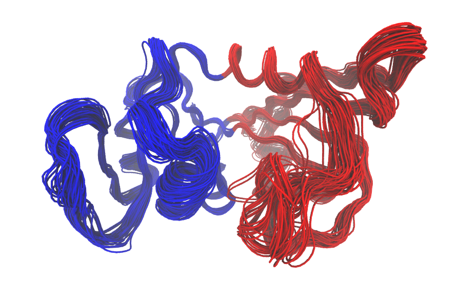
Visualization of domain assignment using function geostas() on the first five normal modes of the entire ensemble of 82 DHFR structures.
Measures for modes comparison
Bio3D now includes multiple measures for the assessment of similarity between two normal mode objects. This enables clustering of related proteins based on the predicted modes of motion. Below we demonstrate the use of root mean squared inner product (RMSIP), squared inner product (SIP), covariance overlap, bhattacharyya coefficient, and PCA of the corresponding covariance matrices.
# Similarity of atomic fluctuations
sip <- sip(modes)
hc.sip <- hclust(as.dist(1-sip), method="ward.D2")
grps.sip <- cutree(hc.sip, k=3)
hclustplot(hc.sip, k=3, colors=grps.rd, labels=ids, cex=0.7, main="SIP", fillbox=FALSE)

par(fig=c(.65, 1, .45, 1), new = TRUE)
plot(pc.xray$z[,1:2], col="grey50", pch=16, cex=1.1,
     ylab="", xlab="", axes=FALSE, bg="red")
points(pc.xray$z[,1:2], col=grps.sip, pch=16, cex=0.7)
box()
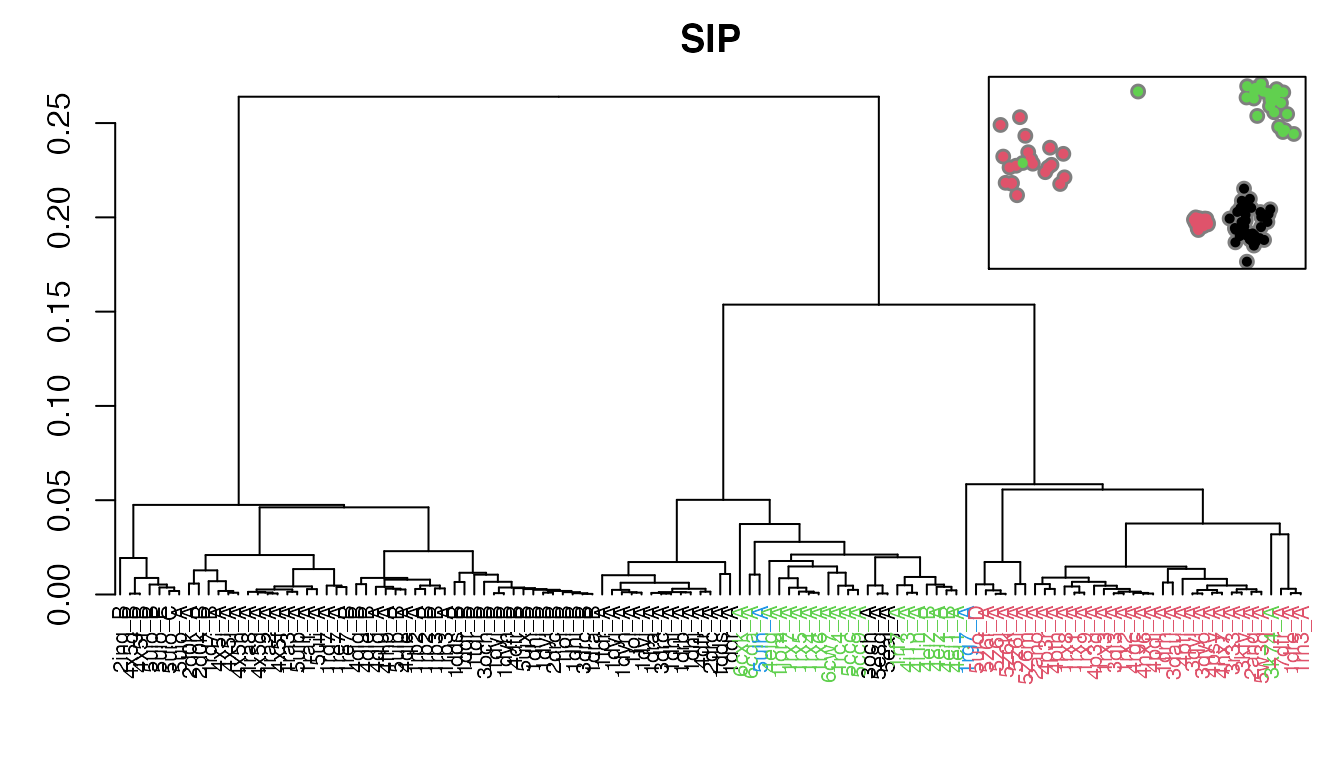
Dendrogram shows the results of hierarchical clustering of structures based on the similarity of atomic fluctuations calculated from NMA. Colors of the labels depict associated conformatial state: green (occluded), black (open), and red (closed). The inset shows the conformerplot (see Figure 2), with colors according to clustering based on pairwise SIP values.
# RMSIP
rmsip <- rmsip(modes)
hc.rmsip <- hclust(dist(1-rmsip), method="ward.D2")
grps.rmsip <- cutree(hc.rmsip, k=3)
hclustplot(hc.rmsip, k=3, colors=grps.rd, labels=ids, cex=0.7, main="RMSIP", fillbox=FALSE)

par(fig=c(.65, 1, .45, 1), new = TRUE)
plot(pc.xray$z[,1:2], col="grey50", pch=16, cex=1.1,
     ylab="", xlab="", axes=FALSE)
points(pc.xray$z[,1:2], col=grps.rmsip, pch=16, cex=0.7)
box()
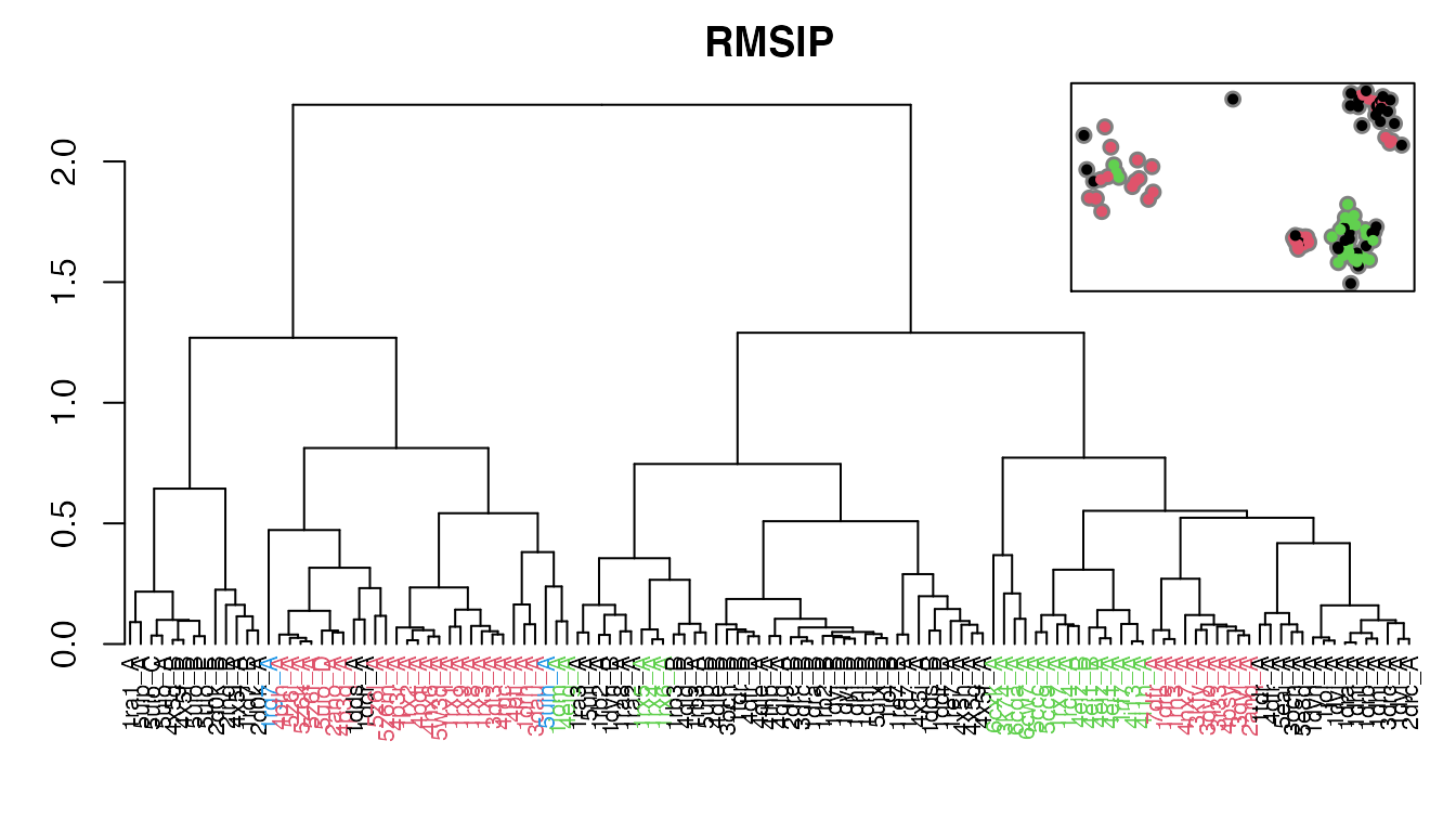
Dendrogram shows the results of hierarchical clustering of structures based on their pairwise RMSIP values (calculated from NMA). Colors of the labels depict associated conformatial state: green (occluded), black (open), and red (closed). The inset shows the conformerplot (see Figure 2), with colors according to clustering based on the pairwise RMSIP values.
# Covariance overlap
co <- covsoverlap(modes, subset=200)
hc.co <- hclust(as.dist(1-co), method="ward.D2")
grps.co <- cutree(hc.co, k=3)
hclustplot(hc.co, k=3, colors=grps.rd, labels=ids, cex=0.7, main="Covariance overlap", fillbox=FALSE)

par(fig=c(.65, 1, .45, 1), new = TRUE)
plot(pc.xray$z[,1:2], col="grey50", pch=16, cex=1.1,
     ylab="", xlab="", axes=FALSE)
points(pc.xray$z[,1:2], col=grps.co, pch=16, cex=0.7)
box()
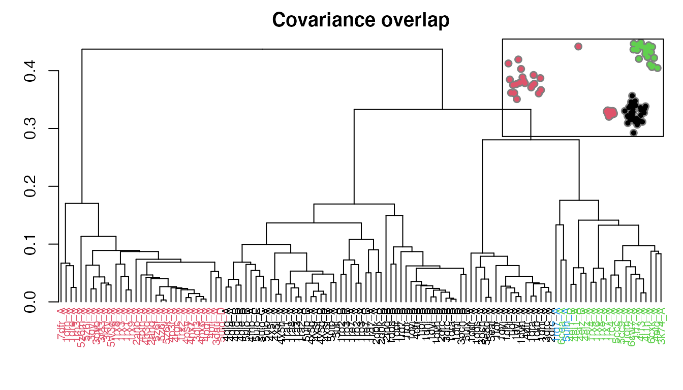
Dendrogram shows the results of hierarchical clustering of structures based on their pairwise covariance overlap (calculated from NMA). Colors of the labels depict associated conformatial state: green (occluded), black (open), and red (closed). The inset shows the conformerplot (see Figure 2), with colors according to clustering of the Covariance overlap measure.
# Bhattacharyya coefficient
covs <- cov.enma(modes)
bc <- bhattacharyya(modes, covs=covs)
hc.bc <- hclust(dist(1-bc), method="ward.D2")
grps.bc <- cutree(hc.bc, k=3)
hclustplot(hc.bc, k=3, colors=grps.rd, labels=ids, cex=0.7, main="Bhattacharyya coefficient", fillbox=FALSE)

par(fig=c(.65, 1, .45, 1), new = TRUE)
plot(pc.xray$z[,1:2], col="grey50", pch=16, cex=1.1,
     ylab="", xlab="", axes=FALSE)
points(pc.xray$z[,1:2], col=grps.bc, pch=16, cex=0.7)
box()
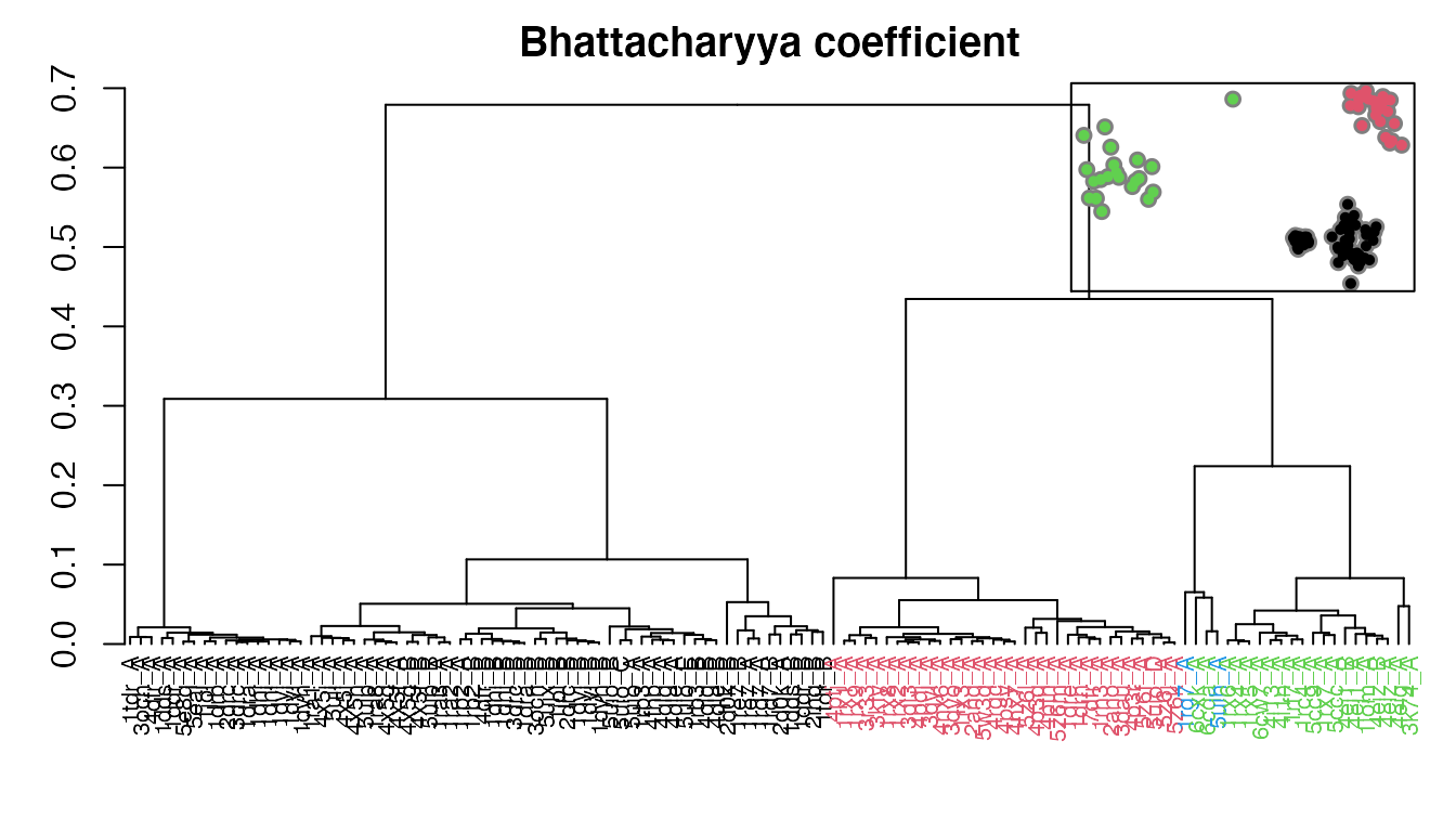
Dendrogram shows the results of hierarchical clustering of structures based on their pairwise Bhattacharyya coefficient (calculated from NMA). Colors of the labels depict associated conformatial state: green (occluded), black (open), and red (closed). The inset shows the conformerplot (see Figure 2), with colors according to clustering of the pairwise Bhattacharyya coefficients.
# PCA of covariance matrices
pc.covs <- pca.array(covs)
hc.covs <- hclust(dist(pc.covs$z[,1:2]), method="ward.D2")
grps.covs <- cutree(hc.covs, k=3)
hclustplot(hc.covs, k=3, colors=grps.rd, labels=ids, cex=0.7, main="PCA of covariance matrices", fillbox=FALSE)

par(fig=c(.65, 1, .45, 1), new = TRUE)
plot(pc.xray$z[,1:2], col="grey50", pch=16, cex=1.1,
     ylab="", xlab="", axes=FALSE)
points(pc.xray$z[,1:2], col=grps.covs, pch=16, cex=0.7)
box()
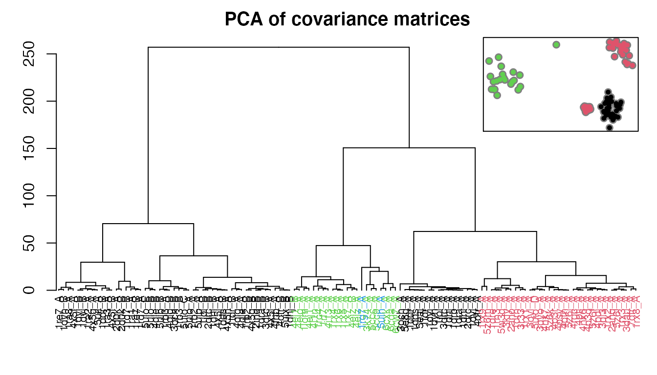
Dendrogram shows the results of hierarchical clustering of structures based on the PCA of covariance matrices (calculated from NMA). Colors of the labels depict associated conformatial state: green (occluded), black (open), and red (closed). The inset shows the conformerplot (see Figure 2), with colors according to clustering based on PCA of covariance matrices.
Document Details
This document is shipped with the Bio3D package in both R and PDF formats. All code can be extracted and automatically executed to generate Figures and/or the PDF with the following commands:
Information About the Current Bio3D Session
print(sessionInfo(), FALSE)
## R version 4.0.2 (2020-06-22)
## Platform: x86_64-apple-darwin17.0 (64-bit)
## Running under: macOS Catalina 10.15.6
##
## Matrix products: default
## BLAS:   /Library/Frameworks/R.framework/Versions/4.0/Resources/lib/libRblas.dylib
## LAPACK: /Library/Frameworks/R.framework/Versions/4.0/Resources/lib/libRlapack.dylib
##
## attached base packages:
## [1] stats     graphics  grDevices utils     datasets  methods   base
##
## other attached packages:
## [1] bio3d.nma_0.1.0.9000 bio3d_2.4-1.9000
##
## loaded via a namespace (and not attached):
##  [1] Rcpp_1.0.5         cpp11_0.2.1        knitr_1.29         magrittr_1.5
##  [5] lattice_0.20-41    R6_2.4.1           ragg_0.3.1         rlang_0.4.7
##  [9] highr_0.8          stringr_1.4.0      tools_4.0.2        parallel_4.0.2
## [13] grid_4.0.2         xfun_0.17          KernSmooth_2.23-17 htmltools_0.5.0
## [17] systemfonts_0.3.1  yaml_2.2.1         assertthat_0.2.1   rprojroot_1.3-2
## [21] digest_0.6.25      pkgdown_1.6.1.9000 crayon_1.3.4       fs_1.5.0
## [25] ncdf4_1.17         memoise_1.1.0      evaluate_0.14      rmarkdown_2.3
## [29] stringi_1.5.3      compiler_4.0.2     desc_1.2.0         backports_1.1.9
References
Grant, B. J., A. P. D. C Rodrigues, K. M. Elsawy, A. J. Mccammon, and L. S. D. Caves. 2006. “Bio3d: An R Package for the Comparative Analysis of Protein Structures.” Bioinformatics 22: 2695–6. https://doi.org/10.1093/bioinformatics/btl461.
Romanowska, Julia, Krzysztof S. Nowinski, and Joanna Trylska. 2012. “Determining geometrically stable domains in molecular conformation sets.” Journal of Chemical Theory and Computation 8 (8): 2588–99. https://doi.org/10.1021/ct300206j.
Skjaerven, L., X. Q. Yao, G. Scarabelli, and B. J. Grant. 2015. “Integrating Protein Structural Dynamics and Evolutionary Analysis with Bio3d.” BMC Bioinformatics 15: 399. https://doi.org/10.1186/s12859-014-0399-6.
The latest version of the package, full documentation and further vignettes (including detailed installation instructions) can be obtained from the main Bio3D website: http://thegrantlab.org/bio3d/↩︎
This vignette contains executable examples, see
help(vignette)for further details.↩︎