Getting started with Bio3D
Lars Skjaerven, Xin-Qiu Yao & Barry J. Grant
Bio3D_introduction.RmdIntroduction
Bio3D1 is a group of R packages containing utilities for the analysis of biomolecular structure, sequence and trajectory data (Grant et al. 2006). Features include the ability to read and write biomolecular structure, sequence and dynamic trajectory data, perform atom selection, re-orientation, superposition, rigid core identification, clustering, distance matrix analysis, conservation analysis, normal mode analysis and principal component analysis. Bio3D takes advantage of the extensive graphical and statistical capabilities of the R environment and thus represents a useful framework for exploratory analysis of structural data.
The functionality for various complex analysis tasks is packed in separate Bio3D packages, including:
bio3d (the core package) for data processing and basic analysis, including alignment, sequence and structure comparisons, and inter-conformer analysis with PCA.
bio3d.nma for ensemble normal mode analysis aimed at predicting and contrasting functional dynamics across protein families.
bio3d.cna for protein structure and correlation network analysis to characterize correlated protein motions underlying allosteric regulation.
bio3d.web for enabling user-friendly online interactive analysis of protein structures and their dynamics.
bio3d.eddm for ensemble difference distance matrix analysis approach to characterizing functionally significant conformational changes.
bio3d.view (in development) for interactive 3D visualization.
Using this vignette
The aim of this document, termed a vignette2 in R parlance, is to provide a brief overview of Bio3D. A number of other Bio3D package vignettes are available, including:
At the time of writing these include3:
Installation Prerequisites
Before you attempt to install Bio3D packages you should have a relatively recent version of R installed and working on your system. Detailed instructions for obtaining and installing R on various platforms can be found on the R home page.
Do I need to know R?
To get the most out of Bio3D you should be quite familiar with basic R usage. There are several on–line resources that can help you get started using R. Some of our favorite learning resources are listed in our FAQ.
Essentially, once you have mastered basic vectors, lists and matrices in R you should feel confident about getting stuck into using the Bio3D package.
Additional utilities
There are a number of additional packages and programs that will either interface with Bio3D or that we consider generally invaluable for working with biomolecular structure (e.g. VMD or PyMOL) and sequence (e.g. Seaview) data. A brief description of how to obtain these additional packages is given below.
Bio3D development
We are always interested in adding additional functionality to Bio3D. If you have ideas, suggestions or code that you would like to distribute as part of this package, please contact us. You are also encouraged to contribute your code or issues directly to our bitbucket repository for incorporation into the development version of the package. Please do get in touch – we would like to hear from you!
Getting started
Start R (type R at the command prompt or, on Windows, double click on the R icon) or simply launch RStudio. Then load a Bio3D package, e.g. the core bio3d package, by typing library(bio3d) at the R console prompt.
Then use the command lbio3d() and help() to list the functions within the package
Finding Help
To get help on a particular function try ?function or help(function). For example, ?pca.xyz
?pca.xyz
To search the help system for documentation matching a particular word or topic use the command help.search("topic"). For example, help.search("pdb")
help.search("pdb")
Typing help.start() will start a local HTML interface. After initiating help.start() in a session the ?function commands will open as HTML pages. To execute examples for a particular function use the command example(function). To run examples for the read.dcd function try example(read.dcd)
Bio3d Demo
Run the command demo(bio3d) to obtain a quick overview.
demo(bio3d)
The bio3d package consists of input/output functions, conversion and manipulation functions, analysis functions, and graphics functions all of which are fully documented. Remember that you can get help on any particular function by using the command ?function or help(function) from within R.
help(pca.xyz)
Example Function Usage
To better understand how a particular function operates it is often helpful to view and execute an example. Every function within the Bio3D packages is documented with example code that you can view by issuing the help command.
Running the command example(function) will directly execute the example for a given function. In addition, a number of worked examples are available as short Tutorials on the Bio3D website.
example(plot.bio3d)
Basic usage
Read a PDB file
The main function for reading PDB format coordinate files is called read.pdb(). You can provide input in a number of ways including a local file name or by simply specifying a 4-character PDB database accession code as in this example.
pdb <- read.pdb("1hel")
## Note: Accessing on-line PDB fileprint(pdb)
##
##  Call:  read.pdb(file = "1hel")
##
##    Total Models#: 1
##      Total Atoms#: 1186,  XYZs#: 3558  Chains#: 1  (values: A)
##
##      Protein Atoms#: 1001  (residues/Calpha atoms#: 129)
##      Nucleic acid Atoms#: 0  (residues/phosphate atoms#: 0)
##
##      Non-protein/nucleic Atoms#: 185  (residues: 185)
##      Non-protein/nucleic resid values: [ HOH (185) ]
##
##    Protein sequence:
##       KVFGRCELAAAMKRHGLDNYRGYSLGNWVCAAKFESNFNTQATNRNTDGSTDYGILQINS
##       RWWCNDGRTPGSRNLCNIPCSALLSSDITASVNCAKKIVSDGNGMNAWVAWRNRCKGTDV
##       QAWIRGCRL
##
## + attr: atom, xyz, seqres, helix, sheet,
##         calpha, remark, call
Just typing your new object name (here we called it pdb) will also call this dedicated print.pdb() function to provide the overview information above.
If you want to finer grained access to the actual data within these files you can access different components of the returned list object. For example:
head(pdb$atom)
##   type eleno elety  alt resid chain resno insert      x      y      z o     b
## 1 ATOM     1     N <NA>   LYS     A     1   <NA>  3.294 10.164 10.266 1 11.18
## 2 ATOM     2    CA <NA>   LYS     A     1   <NA>  2.388 10.533  9.168 1  9.68
## 3 ATOM     3     C <NA>   LYS     A     1   <NA>  2.438 12.049  8.889 1 14.00
## 4 ATOM     4     O <NA>   LYS     A     1   <NA>  2.406 12.898  9.815 1 14.00
## 5 ATOM     5    CB <NA>   LYS     A     1   <NA>  0.949 10.101  9.559 1 13.29
## 6 ATOM     6    CG <NA>   LYS     A     1   <NA> -0.050 10.621  8.573 1 13.52
##   segid elesy charge
## 1  <NA>     N   <NA>
## 2  <NA>     C   <NA>
## 3  <NA>     C   <NA>
## 4  <NA>     O   <NA>
## 5  <NA>     C   <NA>
## 6 <NA> C <NA>print(pdb$xyz)
##
##    Total Frames#: 1
##    Total XYZs#:   3558,  (Atoms#:  1186)
##
##     [1]  3.294  10.164  10.266  <...>  7.795  26.278  15.645  [3558]
##
## + attr: Matrix DIM = 1 x 3558
You can find out more in subsequent vignettes and tutorials available on the main package website.
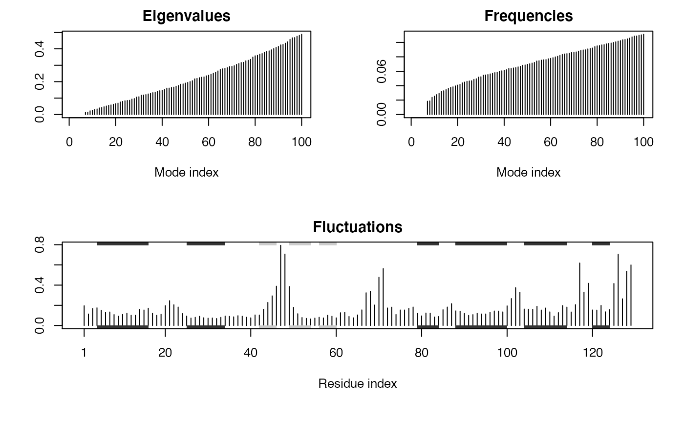
Let’s finish here by doing a quick Normal Mode Analysis (NMA for short)4 to predict the flexibility of this particular structure.
modes <- nma(pdb)
##  Building Hessian...     Done in 0.013 seconds.
## Diagonalizing Hessian... Done in 0.075 seconds.plot(modes)

All package functions have detailed documentation and allow for substantial customization via fully documented input arguments. For example, let’s add some secondary structure annotation taken from the PDB file to the fluctuation plot we just obtained above. This will add marginal rectangles for alpha helix and beta strand regions (in black and gray by default):
plot(modes, sse=pdb)
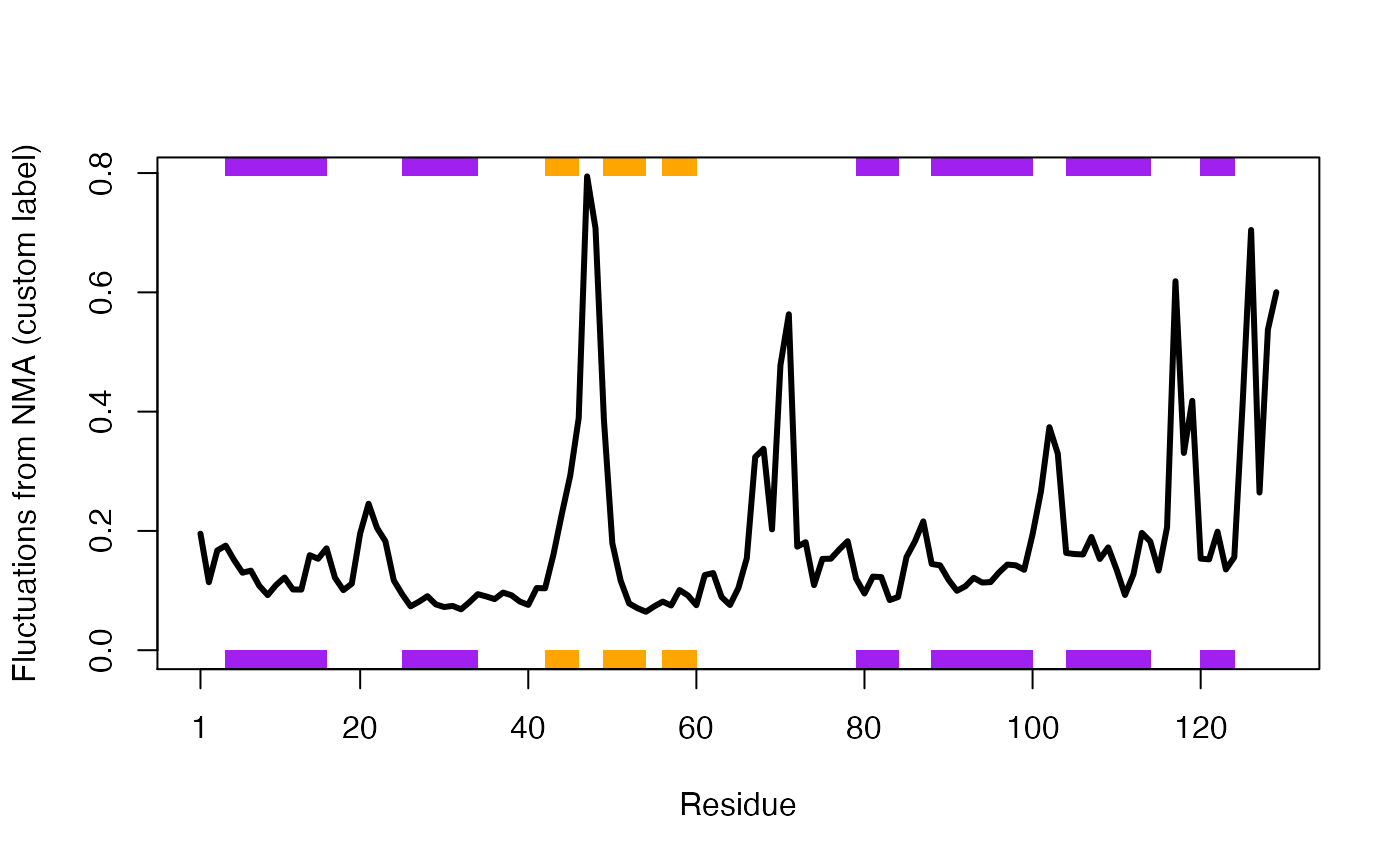
You can quickly take this customization too far ;-)
plot.bio3d(modes$fluctuations, sse=pdb, sheet.col="orange", helix.col="purple", typ="l", lwd=3, ylab="Fluctuations from NMA (custom label)")
Document Details
This document is available from the Bio3D website in R markdown, HTML, and PDF formats. All code can be extracted and automatically executed to generate Figures and/or the PDF with the following commands:
Information About the Current Bio3D Session
## R version 4.0.2 (2020-06-22)
## Platform: x86_64-apple-darwin17.0 (64-bit)
## Running under: macOS Catalina 10.15.6
##
## Matrix products: default
## BLAS:   /Library/Frameworks/R.framework/Versions/4.0/Resources/lib/libRblas.dylib
## LAPACK: /Library/Frameworks/R.framework/Versions/4.0/Resources/lib/libRlapack.dylib
##
## locale:
## [1] en_US.UTF-8/en_US.UTF-8/en_US.UTF-8/C/en_US.UTF-8/en_US.UTF-8
##
## attached base packages:
## [1] stats     graphics  grDevices utils     datasets  methods   base
##
## other attached packages:
## [1] bio3d_2.4-1.9000
##
## loaded via a namespace (and not attached):
##  [1] Rcpp_1.0.5         digest_0.6.25      crayon_1.3.4       rprojroot_1.3-2
##  [5] assertthat_0.2.1   grid_4.0.2         R6_2.4.1           backports_1.1.9
##  [9] magrittr_1.5       evaluate_0.14      stringi_1.5.3      rlang_0.4.7
## [13] fs_1.5.0           ragg_0.3.1         rmarkdown_2.3      pkgdown_1.6.1.9000
## [17] desc_1.2.0         tools_4.0.2        stringr_1.4.0      parallel_4.0.2
## [21] yaml_2.2.1         xfun_0.17          compiler_4.0.2     systemfonts_0.3.1
## [25] cpp11_0.2.1        memoise_1.1.0      htmltools_0.5.0    knitr_1.29
References
Grant, B. J., A. P. D. C Rodrigues, K. M. Elsawy, A. J. Mccammon, and L. S. D. Caves. 2006. “Bio3d: An R Package for the Comparative Analysis of Protein Structures.” Bioinformatics 22: 2695–6. https://doi.org/10.1093/bioinformatics/btl461.
The latest version of the package, full documentation and further vignettes (including detailed installation instructions) can be obtained from the main Bio3D website: thegrantlab.org/bio3d/.↩︎
This vignette contains executable examples, see
help(vignette)for further details.↩︎See also dedicated vignettes for ensemble NMA provided with the Bio3D package.↩︎
See also dedicated vignettes for ensemble NMA provided with the Bio3D package.↩︎