Reconstruction of the Girvan-Newman Community Tree for a CNA Class Object.
community.tree.RdThis function reconstructs the community tree of the community clustering analysis performed by the ‘cna’ function. It allows the user to explore different network community partitions.
community.tree(x, rescale=FALSE)
Arguments
| x | A protein network graph object as obtained from the ‘cna’ function. |
|---|---|
| rescale | Logical, indicating whether to rescale the community names starting from 1. If FALSE, the community names will start from N+1, where N is the number of nodes. |
Value
Returns a list object that includes the following components:
A numeric vector containing the modularity values.
A numeric matrix containing in each row the community residue memberships corresponding to a modularity value. The rows are ordered according to the ‘modularity’ object.
A numeric vector containing the number of communities per modularity value. The vector elements are ordered according to the ‘modularity’ object.
Details
The input of this function should be a ‘cna’ class object containing ‘network’ and ‘communities’ attributes.
This function reconstructs the community residue memberships for each modularity value. The purpose is to facilitate inspection of alternate community partitioning points, which in practice often corresponds to a value close to the maximum of the modularity, but not the maximum value itself.
Author
Guido Scarabelli
See also
Examples
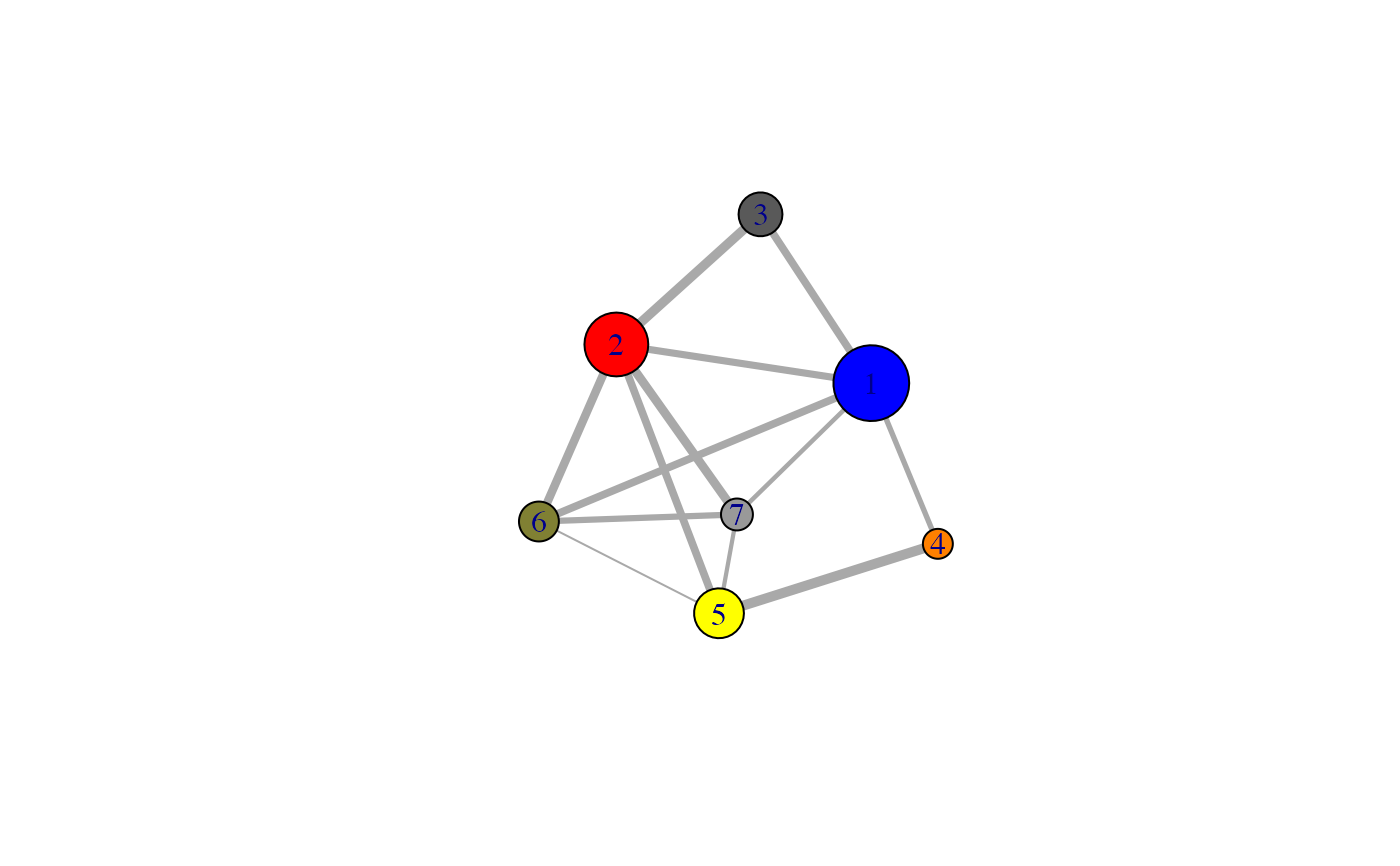
# \donttest{ # PDB server connection required - testing excluded if (!requireNamespace("igraph", quietly = TRUE)) { message('Need igraph installed to run this example') } else { ###-- Build a CNA object pdb <- read.pdb("4Q21") modes <- nma(pdb) cij <- dccm(modes) net <- cna(cij, cutoff.cij=0.2) ##-- Reconstruct the community membership vector for each clustering step. tree <- community.tree(net, rescale=TRUE) ## Plot modularity vs number of communities plot( tree$num.of.comms, tree$modularity ) ## Inspect the maximum modularity value partitioning max.mod.ind <- which.max(tree$modularity) ## Number of communities (k) at max modularity tree$num.of.comms[ max.mod.ind ] ## Membership vector at this partition point tree$tree[max.mod.ind,] # Should be the same as that contained in the original CNA network object net$communities$membership == tree$tree[max.mod.ind,] # Inspect a new membership partitioning (at k=7) memb.k7 <- tree$tree[ tree$num.of.comms == 7, ] ## Produce a new k=7 community network net.7 <- network.amendment(net, memb.k7) plot(net.7, pdb) #view.cna(net.7, trim.pdb(pdb, atom.select(pdb,"calpha")), launch=TRUE ) }#> Note: Accessing on-line PDB file#> Warning: /var/folders/xf/qznxnpf91vb1wm4xwgnbt0xr0000gn/T//Rtmp9oBdbc/4Q21.pdb exists. Skipping download#> Building Hessian... Done in 0.019 seconds. #> Diagonalizing Hessian... Done in 0.183 seconds. #> | |==================================================== | 74% | |==================================================== | 75% | |===================================================== | 75% | |===================================================== | 76% | |====================================================== | 77% | |====================================================== | 78% | |======================================================= | 78% | |======================================================= | 79% | |======================================================== | 79% | |======================================================== | 80% | |======================================================== | 81% | |========================================================= | 81% | |========================================================= | 82% | |========================================================== | 82% | |========================================================== | 83% | |=========================================================== | 84% | |=========================================================== | 85% | |============================================================ | 85% | |============================================================ | 86% | |============================================================= | 86% | |============================================================= | 87% | |============================================================= | 88% | |============================================================== | 88% | |============================================================== | 89% | |=============================================================== | 89% | |=============================================================== | 90% | |=============================================================== | 91% | |================================================================ | 91% | |================================================================ | 92% | |================================================================= | 92% | |================================================================= | 93% | |================================================================= | 94% | |================================================================== | 94% | |================================================================== | 95% | |=================================================================== | 95% | |=================================================================== | 96% | |==================================================================== | 97% | |==================================================================== | 98% | |===================================================================== | 98% | |===================================================================== | 99% | |======================================================================| 99% | |======================================================================| 100%#> Warning: At community.c:460 :Membership vector will be selected based on the lowest modularity score.#> Warning: At community.c:467 :Modularity calculation with weighted edge betweenness community detection might not make sense -- modularity treats edge weights as similarities while edge betwenness treats them as distances#> Obtaining layout from PDB structure# }