Background

Bio3D¹ is an R package that provides interactive tools for structural bioinformatics. The primary focus of Bio3D is the analysis of bimolecular structure, sequence and simulation data (Grant et al. 2006).

Normal mode analysis (NMA) is one of the major simulation techniques used to probe large-scale motions in biomolecules. Typical application is for the prediction of functional motions in proteins. Version 2.0 of the Bio3D package now includes extensive NMA facilities (Skjaerven et al. 2015). These include a unique collection of multiple elastic network model force-fields, automated ensemble analysis methods, and variance weighted NMA (see also the NMA Vignette). Here we provide an in-depth demonstration of ensemble NMA with working code that comprise complete executable examples².

Requirements

Detailed instructions for obtaining and installing the Bio3D package on various platforms can be found in the Installing Bio3D Vignette available both on-line and from within the Bio3D package. In addition to Bio3D the MUSCLE and CLUSTALO multiple sequence alignment programs (available from the muscle home page and clustalo home page) must be installed on your system and in the search path for executables. Please see the installation vignette for further details.

About this document

This vignette was generated using Bio3D version 2.3.0.

Part II: Ensemble NMA across multiple species of DHFR

In this vignette we extend the analysis from Part I by including a more extensive search of distant homologues within the DHFR family. Based on a HMMER search we identify and collect protein species down to a pairwise sequence identity of 20%. Normal modes analysis (NMA) across these species reveals a remarkable similarity of the fluctuation profiles, but also features which are characteristic to specific species.

HMMER search for distantly related DHFR species

Below we use the sequence of E.coli DHFR to perform an initial search against the Pfam HMM database with function hmmer(). The arguments type and db specifies the type of hmmer search and the database to search, respectively. In this particular example, our query sequence is searched against the Pfam profile HMM library (arguments type="hmmscan" and db="pfam") to identify its respecitve protein family. The to hmmer() will return a data frame object containing the Pfam accession ID ($acc), description of the identified family ($desc), family name ($name), etc.

library(bio3d)

# get sequence of Ecoli DHFR
seq <- get.seq("1rx2_A")

## Warning in get.seq("1rx2_A"): Removing existing file: seqs.fasta

# scan the Pfam database for our sequence
pfam <- hmmer(seq, type="hmmscan", db="pfam")
pfam$hit.tbl

Sidenote: The hmmer() function facilitates four different types of searches at a multitude of databases. Use function help(hmmer) for a complete overview of the different options.

Having identified the Pfam entry of our query protein we can use function pfam() to fetch the curated sequence alignment of the DHFR family. Use function print.fasta() to print a short summary of the downloaded sequence alignment to the screen. Note that if argument alignment=TRUE the sequence alignmenment itself will be written to screen.

# download pfam alignment for the DHFR family
pfam.aln <- pfam(pfam$hit.tbl$acc[1])
print(pfam.aln, alignment=FALSE)

## 
## Call:
##   pfam(id = pfam$hit.tbl$acc[1])
## 
## Class:
##   fasta
## 
## Alignment dimensions:
##   60 sequence rows; 208 position columns (114 non-gap, 94 gap) 
## 
## + attr: id, ali, call

The next hmmer search builds a profile HMM from the Pfam multiple sequence alignment and uses this HMM to search against a target sequence database (use type="hmmsearch"). In this case our target sequence database is the PDB (db="pdb"), but there are also other options such as "swissprot" and "uniprot".

# use Pfam alignment in search 
hmm <- hmmer(pfam.aln, type="hmmsearch", db="pdb")

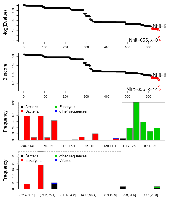
Function plot.hmmer() (the equivalent to plot.blast()) provides a quick overview of the rearch results, and can aid in the identification of a sensible hit similarity threshold. The normalized scores (-log(E-Value)) are shown in the upper panel, and the lower panel provides an overview of the kingdom and specie each hit are associated with. Here we specify a cutoff of 56 yielding 655 hits:

hits <- plot(hmm, cutoff=56)

##   * Possible cutoff values:    56 0 
##             Yielding Nhits:    613 655 
## 
##   * Chosen cutoff value of:    56 
##             Yielding Nhits:    613

Side-note: To visualize the hmmer search results in a web-browser go to the URL in the hmm$url attribute:

# view hmmer results in web-browser
print(hmm$url)

## [1] "http://www.ebi.ac.uk/Tools/hmmer/results/0CECDA66-861B-11E6-8111-D20BDCC3747A"

An summary over the hit species can be obtained by investigatin the hmm$hit.tbl$species attribute:

ids <- hits$acc
species <- hmm$hit.tbl$species[hits$inds]

# print collected species
print(unique(species))

##  [1] "Geobacillus stearothermophilus"                                                                           
##  [2] "Bacillus anthracis"                                                                                       
##  [3] "Coxiella burnetii"                                                                                        
##  [4] "Bacillus anthracis str. Sterne"                                                                           
##  [5] "Moritella profunda"                                                                                       
##  [6] "Yersinia pestis CO92"                                                                                     
##  [7] "Klebsiella pneumoniae CG43"                                                                               
##  [8] "Escherichia coli (strain K12)"                                                                            
##  [9] "Escherichia coli str. K-12 substr. MC4100"                                                                
## [10] "Escherichia coli (GCA_001262935)"                                                                         
## [11] "Escherichia coli str. K-12 substr. DH10B"                                                                 
## [12] "Enterococcus faecalis V583"                                                                               
## [13] "Staphylococcus aureus"                                                                                    
## [14] "Escherichia coli UTI89"                                                                                   
## [15] "Staphylococcus aureus MUF168"                                                                             
## [16] "Staphylococcus aureus RF122"                                                                              
## [17] "Staphylococcus aureus (strain bovine RF122 / ET3-1)"                                                      
## [18] "Staphylococcus aureus (GCA_001353695)"                                                                    
## [19] "Streptococcus pneumoniae"                                                                                 
## [20] "Lactobacillus casei"                                                                                      
## [21] "Mycobacterium tuberculosis (GCA_000735835)"                                                               
## [22] "Mycobacterium tuberculosis"                                                                               
## [23] "Mycobacterium avium"                                                                                      
## [24] "Mycobacterium tuberculosis H37Rv"                                                                         
## [25] "synthetic construct"                                                                                      
## [26] "Klebsiella pneumoniae (GCA_000763925)"                                                                    
## [27] "Haloferax volcanii"                                                                                       
## [28] "Haloferax volcanii (strain ATCC 29605 / DSM 3757 / JCM 8879 / NBRC 14742 / NCIMB 2012 / VKM B-1768 / DS2)"
## [29] "Schistosoma mansoni"                                                                                      
## [30] "Gallus gallus"                                                                                            
## [31] "Mus musculus"                                                                                             
## [32] "Pneumocystis carinii"                                                                                     
## [33] "Homo sapiens"                                                                                             
## [34] "Cryptosporidium hominis"                                                                                  
## [35] "Candida albicans"                                                                                         
## [36] "Candida glabrata CBS 138"                                                                                 
## [37] "Candida glabrata"                                                                                         
## [38] "Toxoplasma gondii"                                                                                        
## [39] "Babesia bovis T2Bo"                                                                                       
## [40] "Babesia bovis"                                                                                            
## [41] "Plasmodium vivax"                                                                                         
## [42] "Plasmodium falciparum"                                                                                    
## [43] "Plasmodium falciparum Vietnam Oak-Knoll (FVO)"                                                            
## [44] "Toxoplasma gondii (strain ATCC 50861 / VEG)"                                                              
## [45] "Plasmodium falciparum VS/1"

Retrieve and process structures from the PDB

Having identified relevant PDB structures through the hmmer search we proceed by fetching and pre-processing the PDB files with functions get.pdb() and pdbsplit().

As in the previous vignette, we are interested in protein structures without missing in-structure residues, and we also want to limit the number of identifical conformers:

# fetch and split PDBs
raw.files <- get.pdb(ids, path = "raw_pdbs", gzip=TRUE)
files <- pdbsplit(raw.files, ids = ids,
                  path = "raw_pdbs/split_chain", ncore=4)
pdbs.all <- pdbaln(files)

# exclude hits with fusion proteins
gaps <- gap.inspect(pdbs.all$ali)
pdbs <- trim(pdbs.all, row.inds=which(gaps$row > 200))

# exclude specific hits
excl.inds <- unlist(lapply(c("5dxv"), grep, pdbs$id))
pdbs <- trim(pdbs, row.inds=-excl.inds)

# exclude structures with missing residues
conn <- inspect.connectivity(pdbs, cut=4.05)
pdbs <- trim(pdbs, row.inds=which(conn))

# exclude conformational redundant structures
rd <- filter.rmsd(pdbs$xyz, cutoff=0.25, fit=TRUE, ncore=4)
pdbs <- trim(pdbs, row.inds=rd$ind)

In this particular case a standard sequence alignment (e.g. through function pdbaln() or seqaln()) is not sufficient for a correct alignment. We will therefore make use of the Pfam profile alignment, and align our selected PDBs to this using argument profile to function seqaln(). Subsequently, we re-read the fasta file, and use function read.fasta.pdb() to obtain aligned C-alpha atom data (including coordinates etc.) for the PDB ensemble:

# align pdbs to Pfam-profile alignment
aln <- seqaln(pdbs, profile=pfam.aln, exefile="clustalo", extra.args="--dealign")

# final alignment will also contain the profile
# store only PDBs in alignment
aln$ali <- aln$ali[1:length(pdbs$id),]
aln$id  <- aln$id[1:length(pdbs$id)]

# re-read PDBs to match the new alignment
pdbs <- read.fasta.pdb(aln)

# exclude gap-only columns
pdbs <- trim(pdbs)

# refit coordinates
pdbs$xyz <- pdbfit(pdbs)

# refit coordinates, and write PDBs to disk
pdbs$xyz <- pdbfit(pdbs, outpath="flsq/")

# fetch IDs again
ids <- basename.pdb(pdbs$id)
species <- hmm$hit.tbl$species[hmm$hit.tbl$acc %in% ids]

# labels for annotating plots
labs <- paste(substr(species, 1,1), ". ", 
              lapply(strsplit(species, " "), function(x) x[2]), sep="")
print(unique(labs))

##  [1] "G. stearothermophilus" "B. anthracis"         
##  [3] "M. profunda"           "Y. pestis"            
##  [5] "K. pneumoniae"         "E. coli"              
##  [7] "E. faecalis"           "S. aureus"            
##  [9] "S. pneumoniae"         "L. casei"             
## [11] "M. tuberculosis"       "M. avium"             
## [13] "H. volcanii"           "S. mansoni"           
## [15] "G. gallus"             "M. musculus"          
## [17] "P. carinii"            "H. sapiens"           
## [19] "C. albicans"           "C. glabrata"

The pdbs object now contains aligned C-alpha atom data, including Cartesian coordinates, residue numbers, residue types, and B-factors. The sequence alignment is also stored by default to the FASTA format file 'aln.fa' (to view this you can use an alignment viewer such as SEAVIEW, see Requirements section above).

Sequence conservation analysis

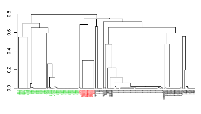
Function seqidentity() can be used to calculate the sequence identity for the PDBs ensemble. Below we also print a summary of the calculated sequence identities, and perform a clustering of the structures based on sequence identity:

seqide <- seqidentity(pdbs)
summary(c(seqide))

##    Min. 1st Qu.  Median    Mean 3rd Qu.    Max. 
##  0.2050  0.3060  0.3290  0.4363  0.3910  1.0000

hc <- hclust(as.dist(1-seqide))
grps.seq <- cutree(hc, h=0.6)

hclustplot(hc, k=3, labels=labs, cex=0.25, fillbox=FALSE)

Normal modes analysis

Function nma.pdbs() will calculate the normal modes of each protein structures stored in the pdbs object. The normal modes are calculated on the full structures as provided by object pdbs. Use argument rm.gaps=FALSE to visualize fluctuations also of un-aligned residues:

modes <- nma(pdbs, rm.gaps=FALSE, ncore=4)

The modes object of class enma contains aligned normal mode data including fluctuations, RMSIP data (only whenrm.gaps=FALSE), and aligned eigenvectors. A short summary of the modes object can be obtain by calling the function print(), and the aligned fluctuations can be plotted with function plot.enma():

print(modes)

## 
## Call:
##   nma.pdbs(pdbs = pdbs, rm.gaps = FALSE, ncore = 4)
## 
## Class:
##   enma
## 
## Number of structures:
##   223
## 
## Attributes stored:
##   - Aligned atomic fluctuations
##   - Aligned eigenvectors (gaps not removed)
##   - Dimensions of x$U.subspace: 720x381x223
## 
## Coordinates were aligned prior to NMA calculations
## 
## + attr: fluctuations, rmsip, U.subspace, L, full.nma, xyz,
##         call

cons <- conserv(pdbs$ali)
sse <- pdbs2sse(pdbs, rm.gaps=FALSE, ind=1)
resno <- pdbs$resno[1, ]
resno[is.na(resno)] <- ""
xlab <- paste0("Residue number (reference PDB: ", basename.pdb(pdbs$id[1]), ")")

par(mfrow=c(2,1), mar=c(4, 4, 2, 2))
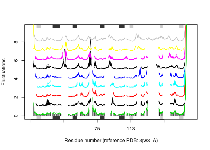
plot(modes, pdbs, ylim=c(0,2), col=grps.seq, label=NULL, xlab=xlab)
plot.bio3d(cons, resno=resno, sse=sse, ylab="Conservation", xlab=xlab)

In some cases it can be difficult to interpret the fluctuation plot when all lines are plotted on top of each other. Argument spread=TRUE adds a small gap between grouped fluctuation profiles. Use this argument in combination with a new groups (grps) variable to function plot.enma():

grps <- rep(NA, length(grps.seq))
grps[grep("coli", labs)]=1
grps[grep("aureus", labs)]=2
grps[grep("anthracis", labs)]=3
grps[grep("tubercu", labs)]=4
grps[grep("casei", labs)]=5
grps[grep("sapiens", labs)]=6
grps[grep("albicans", labs)]=7
grps[grep("glabrata", labs)]=8
grps[grep("carinii", labs)]=9

plot(modes, pdbs=pdbs, col=grps, spread=TRUE, ylim=c(0,1.5), label=NULL)

Visualize modes

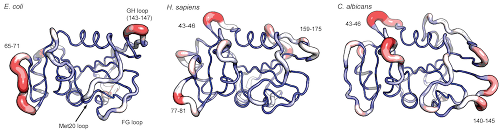
A function call to mktrj.enma() will generate a trajectory PDB file for the visualization of a specific normal mode for one of the structures in the pdbs object. This allows for a visual comparison of the calculated normal modes. Below we make a PDB trajectory of the first mode (argument m.inds=1) of 3 relevant species (e.g. argument s.inds=1). Note that we use grep() to fetch the indices (in the modes and pdbs objects) of the relevant species:

inds <- c(grep("coli", species)[1], 
          grep("sapiens", species)[1],
          grep("albicans", species)[1])

# E.coli
mktrj(modes, pdbs, m.inds=1, s.inds=inds[1], file="ecoli-mode1.pdb")

# H. sapiens
mktrj(modes, pdbs, m.inds=1, s.inds=inds[2], file="hsapiens-mode1.pdb")

# C. albicans
mktrj(modes, pdbs, m.inds=1, s.inds=inds[3], file="calbicans-mode1.pdb")

Document Details

This document is shipped with the Bio3D package in both R and PDF formats. All code can be extracted and automatically executed to generate Figures and/or the PDF with the following commands:

library(rmarkdown)
render("Bio3D_nma-dhfr-partII.Rmd", "all")

Information About the Current Bio3D Session

print(sessionInfo(), FALSE)

## R version 3.3.1 (2016-06-21)
## Platform: x86_64-redhat-linux-gnu (64-bit)
## Running under: Fedora 24 (Twenty Four)
## 
## attached base packages:
## [1] stats     graphics  grDevices utils     datasets  methods   base     
## 
## other attached packages:
## [1] rmarkdown_1.0 bio3d_2.3-0  
## 
## loaded via a namespace (and not attached):
##  [1] magrittr_1.5     formatR_1.4      tools_3.3.1      htmltools_0.3.5 
##  [5] parallel_3.3.1   yaml_2.1.13      Rcpp_0.12.7      codetools_0.2-14
##  [9] stringi_1.1.1    grid_3.3.1       knitr_1.14       stringr_1.0.0   
## [13] digest_0.6.10    evaluate_0.9

References

Grant, B.J., A.P.D.C Rodrigues, K.M. Elsawy, A.J. Mccammon, and L.S.D. Caves. 2006. “Bio3d: An R Package for the Comparative Analysis of Protein Structures.” Bioinformatics 22: 2695–6. doi:10.1093/bioinformatics/btl461.

Skjaerven, L., X.Q. Yao, G. Scarabelli, and B.J. Grant. 2015. “Integrating Protein Structural Dynamics and Evolutionary Analysis with Bio3D.” BMC Bioinformatics 15: 399. doi:10.1186/s12859-014-0399-6.