plot.cmap. bio3d 2.3-0

Usage

"plot"(x, col=2, pch=16, main="Contact map", sub="", xlim=NULL, ylim=NULL, xlab = "Residue index", ylab = xlab,  axes=TRUE, ann=par("ann"), sse=NULL, sse.type="classic", sse.min.length=5, bot=TRUE, left=TRUE, helix.col="gray20", sheet.col="gray80", sse.border=FALSE, add=FALSE, ...)

Arguments

x: a numeric matrix of residue contacts as obtained from function cmap.
col: color code or name, see par.
pch: plotting ‘character’, i.e., symbol to use. This can either be a single character or an integer code for one of a set of graphics symbols. See points.
main: a main title for the plot, see also ‘title’.
sub: a sub-title for the plot.
xlim: the x limits (x1,x2) of the plot. Note that x1 > x2 is allowed and leads to a reversed axis.
ylim: the y limits of the plot.
xlab: a label for the x axis, defaults to a description of ‘x’.
ylab: a label for the y axis, defaults to a description of ‘y’.
axes: a logical value indicating whether both axes should be drawn on the plot. Use graphical parameter ‘xaxt’ or ‘yaxt’ to suppress just one of the axes.
ann: a logical value indicating whether the default annotation (title and x and y axis labels) should appear on the plot.
sse: secondary structure object as returned from dssp, stride or in certain cases read.pdb.
sse.type: single element character vector that determines the type of secondary structure annotation drawn. The following values are possible, ‘classic’ and ‘fancy’. See details and examples below.
sse.min.length: a single numeric value giving the length below which secondary structure elements will not be drawn. This is useful for the exclusion of short helix and strand regions that can often crowd these forms of plots.
left: logical, if TRUE rectangles for each sse are drawn towards the left of the plotting region.
bot: logical, if TRUE rectangles for each sse are drawn towards the bottom of the plotting region.
helix.col: The colors for rectangles representing alpha helices.
sheet.col: The colors for rectangles representing beta strands.
sse.border: The border color for all sse rectangles.
add: logical, specifying if the contact map should be added to an already existing plot. Note that when ‘TRUE’ only points are plotted (no annotation).
...: other graphical parameters.

Description

Plot a contact matrix with optional secondary structure in the marginal regions.

Details

This function is useful for plotting a residue-residue contact data for a given protein structure along with a schematic representation of major secondary structure elements.

Two forms of secondary structure annotation are available: so called ‘classic’ and ‘fancy’. The former draws marginal rectangles and has been available within Bio3D from version 0.1. The later draws more ‘fancy’ (and distracting) 3D like helices and arrowed strands.

Value

Called for its effect.

References

Grant, B.J. et al. (2006) Bioinformatics 22, 2695--2696.

Note

Be sure to check the correspondence of your ‘sse’ object with the ‘x’ values being plotted as no internal checks are performed.

Examples


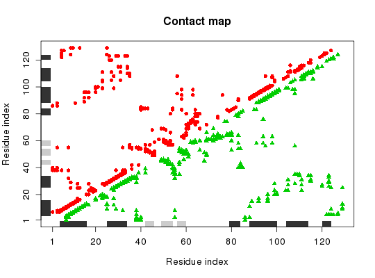
##- Read PDB file
pdb <- read.pdb( system.file("examples/1hel.pdb", package="bio3d") )

##- Calcualte contact map
cm <- cmap(pdb)

##- Plot contact map
plot.cmap(cm, sse=pdb)

##- Add to plot
plot.cmap(t(cm), col=3, pch=17, add=TRUE)

Author

Lars Skjaerven, Barry Grant

Plot Contact Matrix