plot.matrix.loadings. bio3d 2.3-0

Usage

"plot"(x, pc = 1, resno = NULL, sse = NULL, mask.n = 0, ...)

Arguments

x: the results of PCA as obtained from pca.array.
pc: the principal component along which the loadings will be shown.
resno: numerical vector or ‘pdb’ object as obtained from read.pdb to show residue number on the x- and y-axis.
sse: a ‘sse’ object as obtained from dssp or stride, or a ‘pdb’ object as obtained from read.pdb to show secondary structural elements along x- and y-axis.
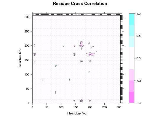
mask.n: the number of elements from the diagonal to be masked from output.
...: additional arguments passed to plot.dccm.

Value

Plot and also returns a numeric matrix containing the loadings.

Description

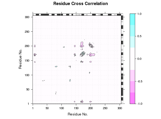
Plot residue-residue matrix loadings of a particular PC that is obtained from a principal component analysis (PCA) of cross-correlation or distance matrices.

Details

The function plots loadings (the eigenvectors) of PCA performed on a set of matrices such as distance matrices from an ensemble of crystallographic structures and residue-residue cross-correlations or covariance matrices derived from ensemble NMA or MD simulation replicates (See pca.array for detail). Loadings are displayed as a matrix with dimension the same as the input matrices of the PCA. Each element of loadings represents the proportion that the corresponding residue pair contributes to the variance in a particular PC. The plot can be used to identify key regions that best explain the variance of underlying matrices.

References

Skjaerven, L. et al. (2014) BMC Bioinformatics 15, 399. Grant, B.J. et al. (2006) Bioinformatics 22, 2695--2696.

Examples

   attach(transducin)
   gaps.res <- gap.inspect(pdbs$ali)
   sse <- bounds.sse(pdbs$sse[1, gaps.res$f.inds])

   # calculate modes
   modes <- nma(pdbs, ncore=NULL)

Warning message:
3QI2_B might have missing residue(s) in structure:
   Fluctuations at neighboring positions may be affected.

Details of Scheduled Calculation:
  ... 53 input structures 
  ... storing 909 eigenvectors for each structure 
  ... dimension of x$U.subspace: ( 915x909x53 )
  ... coordinate superposition prior to NM calculation 
  ... aligned eigenvectors (gap containing positions removed)  
  ... estimated memory usage of final 'eNMA' object: 336.8 Mb 


  |                                                                            
  |                                                                      |   0%


   # calculate cross-correlation matrices from the modes
   cijs <- dccm(modes, ncore=NULL)$all.dccm

   # do PCA on cross-correlation matrices
   pc <- pca.array(cijs)

   # plot loadings
   l <- plot.matrix.loadings(pc, sse=sse)
   l[1:10, 1:10]


              [,1]         [,2]       [,3]         [,4]         [,5]
 [1,]  0.000000000 -0.005377719 0.01655510 -0.009447706  0.008181432
 [2,] -0.005377719  0.000000000 0.06076979  0.043934620  0.057926142
 [3,]  0.016555096  0.060769787 0.00000000  0.015485347  0.060869248
 [4,] -0.009447706  0.043934620 0.01548535  0.000000000  0.064631162
 [5,]  0.008181432  0.057926142 0.06086925  0.064631162  0.000000000
 [6,]  0.013125145  0.048562595 0.06950852  0.081754215  0.097543055
 [7,]  0.047085071  0.048491901 0.03190358 -0.017976973  0.004826396
 [8,]  0.048831159  0.043642856 0.02577068 -0.021062632 -0.036810509
 [9,]  0.031796875  0.044415020 0.03879917  0.019895220  0.044282772
[10,]  0.021439384  0.045968042 0.04997447  0.050303833  0.085480899
             [,6]         [,7]        [,8]        [,9]      [,10]
 [1,]  0.01312514  0.047085071  0.04883116  0.03179688 0.02143938
 [2,]  0.04856259  0.048491901  0.04364286  0.04441502 0.04596804
 [3,]  0.06950852  0.031903576  0.02577068  0.03879917 0.04997447
 [4,]  0.08175421 -0.017976973 -0.02106263  0.01989522 0.05030383
 [5,]  0.09754306  0.004826396 -0.03681051  0.04428277 0.08548090
 [6,]  0.00000000 -0.030343841 -0.05462225  0.07912561 0.08507858
 [7,] -0.03034384  0.000000000 -0.24051981 -0.11044962 0.09159816
 [8,] -0.05462225 -0.240519812  0.00000000  0.05255921 0.02506549
 [9,]  0.07912561 -0.110449617  0.05255921  0.00000000 0.11784389
[10,]  0.08507858  0.091598164  0.02506549  0.11784389 0.00000000


   # plot loadings with elements 10-residue separated from diagonal masked
   plot.matrix.loadings(pc, sse=sse, mask.n=10)

Author

Xin-Qiu Yao

Plot Residue-Residue Matrix Loadings