DCCM Plot

Usage

"plot"(x, resno=NULL, sse=NULL, colorkey=TRUE, at=c(-1, -0.75, -0.5,  -0.25, 0.25, 0.5, 0.75, 1), main="Residue Cross Correlation", helix.col = "gray20", sheet.col = "gray80", inner.box=TRUE, outer.box=FALSE, xlab="Residue No.", ylab="Residue No.", margin.segments=NULL, segment.col=vmd_colors(), segment.min=1, ...)

Arguments

x

a numeric matrix of atom-wise cross-correlations as output by the ‘dccm’ function.

resno

an optional vector with length equal to that of x that will be used to annotate the x- and y-axis. This is typically a vector of residue numbers. Can be also provided with a ‘pdb’ object, in which ‘resno’ of all C-alpha atoms will be used. If NULL residue positions from 1 to the length of x will be used. See examples below.

sse

secondary structure object as returned from dssp, stride or read.pdb.

colorkey

logical, if TRUE a key is plotted.

at

numeric vector specifying the levels to be colored.

main

a main title for the plot.

helix.col

The colors for rectangles representing alpha helices.

sheet.col

The colors for rectangles representing beta strands.

inner.box

logical, if TRUE an outer box is drawn.

outer.box

logical, if TRUE an outer box is drawn.

xlab

a label for the x axis.

ylab

a label for the y axis.

margin.segments

a numeric vector of cluster membership as obtained from cutree() or other community detection method. This will be used for bottom and left margin annotation.

segment.col

a vector of colors used for each cluster group in margin.segments.

segment.min

a single element numeric vector that will cause margin.segments with a length below this value to be excluded from the plot.

...

additional graphical parameters for contourplot.

Examples

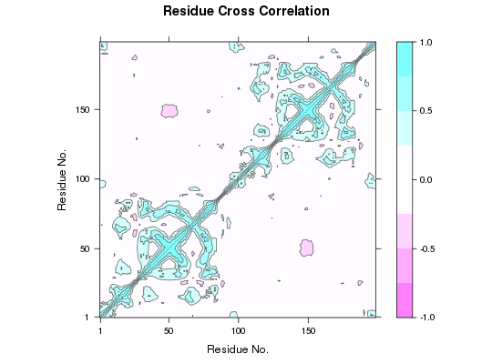
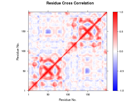
  ##-- Read example trajectory file
  trtfile <- system.file("examples/hivp.dcd", package="bio3d")
  trj <- read.dcd(trtfile)

 NATOM = 198 
 NFRAME= 117 
 ISTART= 0 
 last  = 117 
 nstep = 117 
 nfile = 117 
 NSAVE = 1 
 NDEGF = 0 
 version 24 
Reading (x100)
  |======================================================================| 100%


  ## Read reference PDB and trim it to match the trajectory
  pdb <- trim(read.pdb("1W5Y"), 'calpha')

  Note: Accessing on-line PDB file


  ## select residues 24 to 27 and 85 to 90 in both chains
  inds <- atom.select(pdb, resno=c(24:27,85:90))

  ## lsq fit of trj on pdb
  xyz <- fit.xyz(pdb$xyz, trj, fixed.inds=inds$xyz, mobile.inds=inds$xyz)

  ## Dynamic cross-correlations of atomic displacements
  cij <- dccm(xyz)

  ## Default plot
  plot.dccm(cij)

  ## Change the color scheme and the range of colored data levels
  plot.dccm(cij, contour=FALSE, col.regions=bwr.colors(200), at=seq(-1,1,by=0.01) )




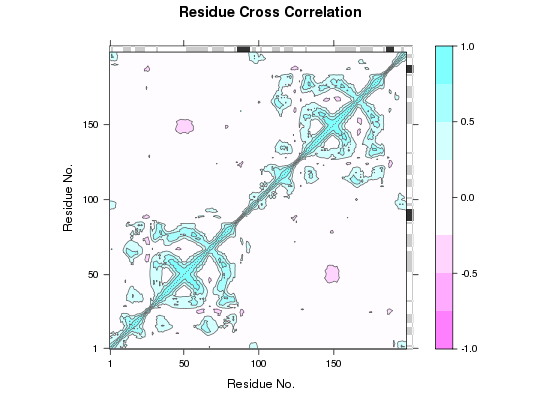
  ## Add secondary structure annotation to plot margins
  plot.dccm(cij, sse=pdb) 



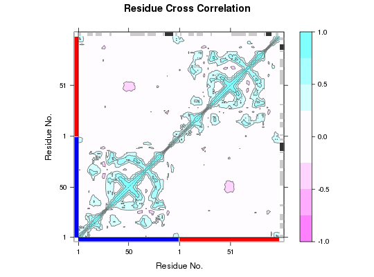
  ## Add additional margin annotation for chains
  ## Also label x- and y-axis with PDB residue numbers
  ch <- ifelse(pdb$atom$chain=="A", 1,2)
  plot.dccm(cij, resno=pdb, sse=pdb, margin.segments=ch)



  ## Plot with cluster annotation from dynamic network analysis
  #net <- cna(cij)
  #plot.dccm(cij, margin.segments=net$raw.communities$membership)

  ## Focus on major communities (i.e. exclude those below a certain total length)
  #plot.dccm(cij, margin.segments=net$raw.communities$membership, segment.min=25)

See also

Author