Protein Dynamic Correlation Network Construction and Community Analysis.
Usage
cna(cij, ...) "cna"(cij, cutoff.cij=0.4, cm=NULL, vnames=colnames(cij), cluster.method="btwn", collapse.method="max", cols=vmd_colors(), minus.log=TRUE, ...) "cna"(cij, ..., ncore = NULL)
Arguments
- cij
- A numeric array with 2 dimensions (nXn) containing atomic correlation values, where "n" is the residue number. The matrix elements should be in between 0 and 1 (atomic correlations). Can be also a set of correlation matrices for ensemble network analysis. See ‘dccm’ function in bio3d package for further details.
- ...
- Additional arguments passed to the methods
cna.dccmandcna.ensmb. - cutoff.cij
- Numeric element specifying the cutoff on cij matrix values. Coupling below cutoff.cij are set to 0.
- cm
- (optinal) A numeric array with 2 dimensions (nXn) containing binary contact values, where "n" is the residue number. The matrix elements should be 1 if two residues are in contact and 0 if not in contact. See the ‘cmap’ function in bio3d package for further details.
- vnames
- A vector of names for each column in the input cij. This will be used for referencing residues in a similar way to residue numbers in later analysis.
- cluster.method
- A character string specifying the method for community determination. Supported methods are: btwn="Girvan-Newman betweenness" walk="Random walk" greed="Greedy algorithm for modularity optimization" infomap="Infomap algorithm for community detection"
- collapse.method
- A single element character vector specifing the ‘cij’ collapse method, can be one of ‘max’, ‘median’, ‘mean’, or ‘trimmed’. By defualt the ‘max’ method is used to collapse the input residue based ‘cij’ matrix into a smaller community based network by taking the maximium ‘abs(cij)’ value between communities as the comunity-to-community cij value for clustered network construction.
- cols
- A vector of colors assigned to network nodes.
- minus.log
- Logical, indicating whether ‘-log(abs(cij))’ values should be used for network construction.
- ncore
- Number of CPU cores used to do the calculation. By default, use all available cores.
Description
This function builds both residue-based and community-based undirected weighted network graphs from an input correlation matrix, as obtained from the functions ‘dccm’, ‘dccm.nma’, and ‘dccm.enma’. Community detection/clustering is performed on the initial residue based network to determine the community organization and network structure of the community based network.
Value
-
Returns a list object that includes igraph network and community
objects with the following components:
- network
- An igraph residue-wise graph object. See below for more details.
- communities
- An igraph residue-wise community object. See below for more details.
- communitiy.network
- An igraph community-wise graph object. See below for more details.
- community.cij
- Numeric square matrix containing the absolute values of the atomic correlation input matrix for each community as obtained from ‘cij’ via application of ‘collapse.method’.
- cij
- Numeric square matrix containing the absolute values of the atomic correlation input matrix.
Details
The input to this function should be a correlation matrix as obtained from the ‘dccm’, ‘dccm.mean’ or ‘dccm.nma’ and related functions. Optionally, a contact map ‘cm’ may also given as input to filter the correlation matrix resulting in the exclusion of network edges between non-contacting atom pairs (as defined in the contact map).
Internally this function calls the igraph package functions ‘graph.adjacency’, ‘edge.betweenness.community’, ‘walktrap.community’, ‘fastgreedy.community’, and ‘infomap.community’. The first constructs an undirected weighted network graph. The second performs Girvan-Newman style clustering by calculating the edge betweenness of the graph, removing the edge with the highest edge betweenness score, calculates modularity (i.e. the difference between the current graph partition and the partition of a random graph, see Newman and Girvan, Physical Review E (2004), Vol 69, 026113), then recalculating edge betweenness of the edges and again removing the one with the highest score, etc. The returned community partition is the one with the highest overall modularity value. ‘walktrap.community’ implements the Pons and Latapy algorithm based on the idea that random walks on a graph tend to get "trapped" into densely connected parts of it, i.e. a community. The random walk process is used to determine a distance between nodes. Nodes with low distance values are joined in the same community. ‘fastgreedy.community’ instead determines the community structure based on the optimization of the modularity. In the starting state each node is isolated and belongs to a separated community. Communities are then joined together (according to the network edges) in pairs and the modularity is calculated. At each step the join resulting in the highest increase of modularity is chosen. This process is repeated until a single community is obtained, then the partitioning with the highest modularity score is selected. ‘infomap.community’ finds community structure that minimizes the expected description length of a random walker trajectory.
Examples
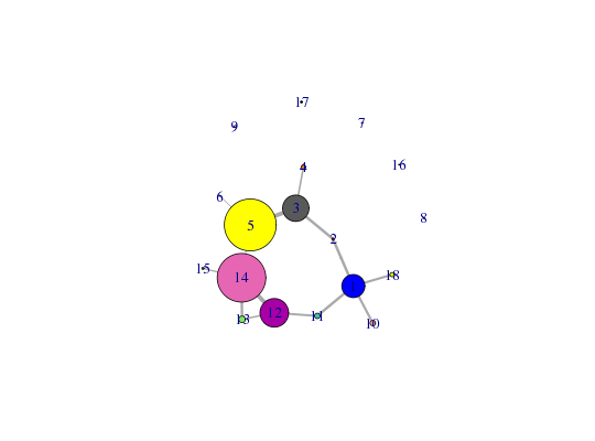
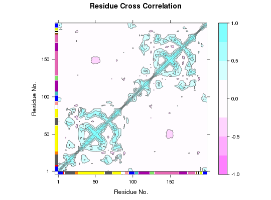
# PDB server connection required - testing excluded ##-- Build a correlation network from NMA results ## Read example PDB pdb <- read.pdb("4Q21")Note: Accessing on-line PDB file## Perform NMA modes <- nma(pdb)Building Hessian... Done in 0.063 seconds. Diagonalizing Hessian... Done in 0.277 seconds.#plot(modes, sse=pdb) ## Calculate correlations cij <- dccm(modes)|======================================================================| 100%#plot(cij, sse=pdb) ## Build, and betweenness cluster, a network graph net <- cna(cij, cutoff.cij=0.35) #plot(net, pdb) ## within VMD set 'coloring method' to 'Chain' and 'Drawing method' to Tube #vmd.cna(net, trim.pdb(pdb, atom.select(pdb,"calpha")), launch=TRUE ) ##-- Build a correlation network from MD results ## Read example trajectory file trtfile <- system.file("examples/hivp.dcd", package="bio3d") trj <- read.dcd(trtfile)NATOM = 198 NFRAME= 117 ISTART= 0 last = 117 nstep = 117 nfile = 117 NSAVE = 1 NDEGF = 0 version 24 Reading (x100) |======================================================================| 100%## Read the starting PDB file to determine atom correspondence pdbfile <- system.file("examples/hivp.pdb", package="bio3d") pdb <- read.pdb(pdbfile) ## select residues 24 to 27 and 85 to 90 in both chains inds <- atom.select(pdb, resno=c(24:27,85:90), elety='CA') ## lsq fit of trj on pdb xyz <- fit.xyz(pdb$xyz, trj, fixed.inds=inds$xyz, mobile.inds=inds$xyz) ## calculate dynamical cross-correlation matrix cij <- dccm(xyz) ## Build, and betweenness cluster, a network graph net <- cna(cij) # Plot coarse grained network based on dynamically coupled communities xy <- plot.cna(net)Obtaining estimated layout with fruchterman.reingoldplot.dccm(cij, margin.segments=net$communities$membership)
##-- Begin to examine network structure - see CNA vignette for more details netCall: cna.dccm(cij = cij) Structure: - NETWORK NODES#: 198 EDGES#: 1841 - COMMUNITY NODES#: 18 EDGES#: 14 + attr: network, communities, community.network, community.cij, cij, callsummary(net)id size members 1 21 c(1:7, 95:102, 193:198) 2 2 8:9 3 24 c(10:23, 63:72) 4 4 24:27 5 47 c(28:62, 73:84) 6 1 85 7 1 86 8 1 87 9 2 88:89 10 5 90:94 11 5 103:107 12 26 c(108:122, 162:172) 13 6 123:128 14 44 c(129:161, 173:183) 15 2 184:185 16 1 186 17 2 187:188 18 4 189:192$id [1] "1" "2" "3" "4" "5" "6" "7" "8" "9" "10" "11" "12" "13" "14" "15" [16] "16" "17" "18" $size 1 2 3 4 5 6 7 8 9 10 11 12 13 14 15 16 17 18 21 2 24 4 47 1 1 1 2 5 5 26 6 44 2 1 2 4 $members $members$`1` 1 2 3 4 5 6 7 95 96 97 98 99 100 101 102 193 194 195 196 197 1 2 3 4 5 6 7 95 96 97 98 99 100 101 102 193 194 195 196 197 198 198 $members$`2` 8 9 8 9 $members$`3` 10 11 12 13 14 15 16 17 18 19 20 21 22 23 63 64 65 66 67 68 69 70 71 72 10 11 12 13 14 15 16 17 18 19 20 21 22 23 63 64 65 66 67 68 69 70 71 72 $members$`4` 24 25 26 27 24 25 26 27 $members$`5` 28 29 30 31 32 33 34 35 36 37 38 39 40 41 42 43 44 45 46 47 48 49 50 51 52 53 28 29 30 31 32 33 34 35 36 37 38 39 40 41 42 43 44 45 46 47 48 49 50 51 52 53 54 55 56 57 58 59 60 61 62 73 74 75 76 77 78 79 80 81 82 83 84 54 55 56 57 58 59 60 61 62 73 74 75 76 77 78 79 80 81 82 83 84 $members$`6` 85 85 $members$`7` 86 86 $members$`8` 87 87 $members$`9` 88 89 88 89 $members$`10` 90 91 92 93 94 90 91 92 93 94 $members$`11` 103 104 105 106 107 103 104 105 106 107 $members$`12` 108 109 110 111 112 113 114 115 116 117 118 119 120 121 122 162 163 164 165 166 108 109 110 111 112 113 114 115 116 117 118 119 120 121 122 162 163 164 165 166 167 168 169 170 171 172 167 168 169 170 171 172 $members$`13` 123 124 125 126 127 128 123 124 125 126 127 128 $members$`14` 129 130 131 132 133 134 135 136 137 138 139 140 141 142 143 144 145 146 147 148 129 130 131 132 133 134 135 136 137 138 139 140 141 142 143 144 145 146 147 148 149 150 151 152 153 154 155 156 157 158 159 160 161 173 174 175 176 177 178 179 149 150 151 152 153 154 155 156 157 158 159 160 161 173 174 175 176 177 178 179 180 181 182 183 180 181 182 183 $members$`15` 184 185 184 185 $members$`16` 186 186 $members$`17` 187 188 187 188 $members$`18` 189 190 191 192 189 190 191 192 $tbl id size members 1 1 21 c(1:7, 95:102, 193:198) 2 2 2 8:9 3 3 24 c(10:23, 63:72) 4 4 4 24:27 5 5 47 c(28:62, 73:84) 6 6 1 85 7 7 1 86 8 8 1 87 9 9 2 88:89 10 10 5 90:94 11 11 5 103:107 12 12 26 c(108:122, 162:172) 13 13 6 123:128 14 14 44 c(129:161, 173:183) 15 15 2 184:185 16 16 1 186 17 17 2 187:188 18 18 4 189:192attributes(net)$names [1] "network" "communities" "community.network" [4] "community.cij" "cij" "call" $class [1] "cna"table( net$communities$members )1 2 3 4 5 6 7 8 9 10 11 12 13 14 15 16 17 18 21 2 24 4 47 1 1 1 2 5 5 26 6 44 2 1 2 4
See also
plot.cna, summary.cna,
vmd.cna, graph.adjacency,
edge.betweenness.community,
walktrap.community,
fastgreedy.community,
infomap.community