###
### Example of PDB file manipulation, searching, alignment etc.
###
### Authors Xin-Qiu Yao
### Lars Skjaerven
### Barry J Grant
###
require(bio3d); require(graphics);
pause <- function() {
cat("Press ENTER/RETURN/NEWLINE to continue.")
readLines(n=1)
invisible()
}
#############################################
## #
## Basic PDB file reading and manipulation #
## #
#############################################
pause()
Press ENTER/RETURN/NEWLINE to continue.
# Read an online RCSB Protein Data Bank structure
pdb <- read.pdb("4q21")
Note: Accessing on-line PDB file
# Whats in the new pdb object
print(pdb)
Call: read.pdb(file = "4q21")
Total Models#: 1
Total Atoms#: 1447, XYZs#: 4341 Chains#: 1 (values: A)
Protein Atoms#: 1340 (residues/Calpha atoms#: 168)
Nucleic acid Atoms#: 0 (residues/phosphate atoms#: 0)
Non-protein/nucleic Atoms#: 107 (residues: 80)
Non-protein/nucleic resid values: [ GDP (1), HOH (78), MG (1) ]
Protein sequence:
MTEYKLVVVGAGGVGKSALTIQLIQNHFVDEYDPTIEDSYRKQVVIDGETCLLDILDTAG
QEEYSAMRDQYMRTGEGFLCVFAINNTKSFEDIHQYREQIKRVKDSDDVPMVLVGNKCDL
AARTVESRQAQDLARSYGIPYIETSAKTRQGVEDAFYTLVREIRQHKL
+ attr: atom, xyz, seqres, helix, sheet,
calpha, remark, call
pause()
Press ENTER/RETURN/NEWLINE to continue.
# Most bio3d functions, including read.pdb(), return list objects
attributes(pdb)
$names
[1] "atom" "xyz" "seqres" "helix" "sheet" "calpha" "remark" "call"
$class
[1] "pdb" "sse"
pdb$atom[1:3, c("resno", "resid", "elety", "x", "y", "z")]
resno resid elety x y z
1 1 MET N 64.080 50.529 32.509
2 1 MET CA 64.044 51.615 33.423
3 1 MET C 63.722 52.849 32.671
pause()
Press ENTER/RETURN/NEWLINE to continue.
# Selection of substructure regions with 'atom.select()'' function
inds <- atom.select(pdb, elety = c("N","CA","C"), resno=4:6)
pdb$atom[inds$atom,]
type eleno elety alt resid chain resno insert x y z o b
25 ATOM 25 N <NA> TYR A 4 <NA> 62.736 60.251 33.384 1 26.38
26 ATOM 26 CA <NA> TYR A 4 <NA> 61.817 61.333 33.161 1 23.42
27 ATOM 27 C <NA> TYR A 4 <NA> 62.492 62.578 33.675 1 25.05
37 ATOM 37 N <NA> LYS A 5 <NA> 62.654 63.574 32.804 1 21.98
38 ATOM 38 CA <NA> LYS A 5 <NA> 63.343 64.814 33.163 1 21.34
39 ATOM 39 C <NA> LYS A 5 <NA> 62.328 65.837 33.628 1 21.86
46 ATOM 46 N <NA> LEU A 6 <NA> 62.263 66.117 34.955 1 19.48
47 ATOM 47 CA <NA> LEU A 6 <NA> 61.321 67.068 35.557 1 18.99
48 ATOM 48 C <NA> LEU A 6 <NA> 62.005 68.430 35.889 1 25.96
segid elesy charge
25 <NA> N <NA>
26 <NA> C <NA>
27 <NA> C <NA>
37 <NA> N <NA>
38 <NA> C <NA>
39 <NA> C <NA>
46 <NA> N <NA>
47 <NA> C <NA>
48 <NA> C <NA>
pause()
Press ENTER/RETURN/NEWLINE to continue.
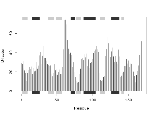
# Simple B-factor plot
ca.inds <- atom.select(pdb, "calpha")
plot.bio3d( pdb$atom[ca.inds$atom,"b"], sse=pdb, ylab="B-factor")
###################################
## #
## Search for similar structures #
## #
###################################
# Use sequence
aa <- pdbseq(pdb)
aa
1 2 3 4 5 6 7 8 9 10 11 12 13 14 15 16 17 18 19 20
"M" "T" "E" "Y" "K" "L" "V" "V" "V" "G" "A" "G" "G" "V" "G" "K" "S" "A" "L" "T"
21 22 23 24 25 26 27 28 29 30 31 32 33 34 35 36 37 38 39 40
"I" "Q" "L" "I" "Q" "N" "H" "F" "V" "D" "E" "Y" "D" "P" "T" "I" "E" "D" "S" "Y"
41 42 43 44 45 46 47 48 49 50 51 52 53 54 55 56 57 58 59 60
"R" "K" "Q" "V" "V" "I" "D" "G" "E" "T" "C" "L" "L" "D" "I" "L" "D" "T" "A" "G"
61 62 63 64 65 66 67 68 69 70 71 72 73 74 75 76 77 78 79 80
"Q" "E" "E" "Y" "S" "A" "M" "R" "D" "Q" "Y" "M" "R" "T" "G" "E" "G" "F" "L" "C"
81 82 83 84 85 86 87 88 89 90 91 92 93 94 95 96 97 98 99 100
"V" "F" "A" "I" "N" "N" "T" "K" "S" "F" "E" "D" "I" "H" "Q" "Y" "R" "E" "Q" "I"
101 102 103 104 105 106 107 108 109 110 111 112 113 114 115 116 117 118 119 120
"K" "R" "V" "K" "D" "S" "D" "D" "V" "P" "M" "V" "L" "V" "G" "N" "K" "C" "D" "L"
121 122 123 124 125 126 127 128 129 130 131 132 133 134 135 136 137 138 139 140
"A" "A" "R" "T" "V" "E" "S" "R" "Q" "A" "Q" "D" "L" "A" "R" "S" "Y" "G" "I" "P"
141 142 143 144 145 146 147 148 149 150 151 152 153 154 155 156 157 158 159 160
"Y" "I" "E" "T" "S" "A" "K" "T" "R" "Q" "G" "V" "E" "D" "A" "F" "Y" "T" "L" "V"
161 162 163 164 165 166 167 168
"R" "E" "I" "R" "Q" "H" "K" "L"
pause()
Press ENTER/RETURN/NEWLINE to continue.
# Blast the RCSB PDB to find similar sequences
blast <- blast.pdb(aa)
Searching ... please wait (updates every 5 seconds) RID = YVBB0DR6015
.
Reporting 319 hits
head(blast$hit.tbl)
queryid subjectids identity positives alignmentlength
1 Query_149033 gi|231226|pdb|6Q21|A 100 100 168
2 Query_149033 gi|231227|pdb|6Q21|B 100 100 168
3 Query_149033 gi|231228|pdb|6Q21|C 100 100 168
4 Query_149033 gi|231229|pdb|6Q21|D 100 100 168
5 Query_149033 gi|15988032|pdb|1IOZ|A 100 100 168
6 Query_149033 gi|157829765|pdb|1AA9|A 100 100 168
mismatches gapopens q.start q.end s.start s.end evalue bitscore
1 0 0 1 168 1 168 1.11e-124 348
2 0 0 1 168 1 168 1.11e-124 348
3 0 0 1 168 1 168 1.11e-124 348
4 0 0 1 168 1 168 1.11e-124 348
5 0 0 1 168 1 168 1.11e-124 348
6 0 0 1 168 1 168 1.11e-124 348
mlog.evalue pdb.id acc
1 285.4162 6Q21_A 231226
2 285.4162 6Q21_B 231227
3 285.4162 6Q21_C 231228
4 285.4162 6Q21_D 231229
5 285.4162 1IOZ_A 15988032
6 285.4162 1AA9_A 157829765
pause()
Press ENTER/RETURN/NEWLINE to continue.
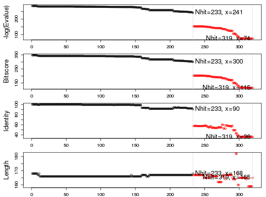
# Plot results
top.hits <- plot(blast)
* Possible cutoff values: 241 74
Yielding Nhits: 233 319
* Chosen cutoff value of: 241
Yielding Nhits: 233
head(top.hits$hits)
pdb.id acc group
1 "6Q21_A" "231226" "1"
2 "6Q21_B" "231227" "1"
3 "6Q21_C" "231228" "1"
4 "6Q21_D" "231229" "1"
5 "1IOZ_A" "15988032" "1"
6 "1AA9_A" "157829765" "1"
pause()
Press ENTER/RETURN/NEWLINE to continue.
## Download and and analyze further ....
## raw.files <- get.pdb(top.hits$pdb.id, path="raw_hits")
## files <- pdbsplit(raw.files, top.hits$hits, path="top_hits")
## pdbs <- pdbaln(files)
## ...<ETC>...