###
### Example of basic molecular dynamics trajectory analysis
###
### Authors Xin-Qiu Yao
### Lars Skjaerven
### Barry J Grant
###
require(bio3d); require(graphics);
pause <- function() {
cat("Press ENTER/RETURN/NEWLINE to continue.")
readLines(n=1)
invisible()
}
#############################################
## #
## Basic analysis of HIVpr trajectory data #
## #
#############################################
pause()
Press ENTER/RETURN/NEWLINE to continue.
# Read example trajectory file
trtfile <- system.file("examples/hivp.dcd", package="bio3d")
trj <- read.dcd(trtfile)
NATOM = 198
NFRAME= 117
ISTART= 0
last = 117
nstep = 117
nfile = 117
NSAVE = 1
NDEGF = 0
version 24
Reading (x100)
|======================================================================| 100%
# Read the starting PDB file to determine atom correspondence
pdbfile <- system.file("examples/hivp.pdb", package="bio3d")
pdb <- read.pdb(pdbfile)
# Whats in the new pdb object
print(pdb)
Call: read.pdb(file = pdbfile)
Total Models#: 1
Total Atoms#: 198, XYZs#: 594 Chains#: 2 (values: A B)
Protein Atoms#: 198 (residues/Calpha atoms#: 198)
Nucleic acid Atoms#: 0 (residues/phosphate atoms#: 0)
Non-protein/nucleic Atoms#: 0 (residues: 0)
Non-protein/nucleic resid values: [ none ]
Protein sequence:
PQITLWQRPLVTIKIGGQLKEALLDTGADDTVLEEMSLPGRWKPKMIGGIGGFIKVRQYD
QILIEICGHKAIGTVLVGPTPVNIIGRNLLTQIGCTLNFPQITLWQRPLVTIKIGGQLKE
ALLDTGADDTVLEEMSLPGRWKPKMIGGIGGFIKVRQYDQILIEICGHKAIGTVLVGPTP
VNIIGRNLLTQIGCTLNF
+ attr: atom, xyz, helix, sheet, calpha,
call
pause()
Press ENTER/RETURN/NEWLINE to continue.
# How many rows (frames) and columns (coords) present in trj
dim(trj)
[1] 117 594
ncol(trj) == length(pdb$xyz)
[1] TRUE
pause()
Press ENTER/RETURN/NEWLINE to continue.
# Trajectory Frame Superposition on Calpha atoms
ca.inds <- atom.select(pdb, elety = "CA")
xyz <- fit.xyz(fixed = pdb$xyz, mobile = trj,
fixed.inds = ca.inds$xyz,
mobile.inds = ca.inds$xyz)
# Root Mean Square Deviation (RMSD)
rd <- rmsd(xyz[1, ca.inds$xyz], xyz[, ca.inds$xyz])
plot(rd, typ = "l", ylab = "RMSD", xlab = "Frame No.")
points(lowess(rd), typ = "l", col = "red", lty = 2, lwd = 2)
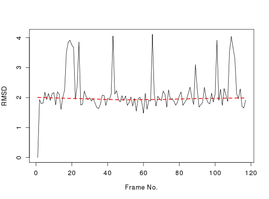
summary(rd)
Min. 1st Qu. Median Mean 3rd Qu. Max.
0.000 1.834 1.967 2.151 2.167 4.112
pause()
Press ENTER/RETURN/NEWLINE to continue.
# Root Mean Squared Fluctuations (RMSF)
rf <- rmsf(xyz[, ca.inds$xyz])
plot(rf, ylab = "RMSF", xlab = "Residue Position", typ="l")

pause()
Press ENTER/RETURN/NEWLINE to continue.
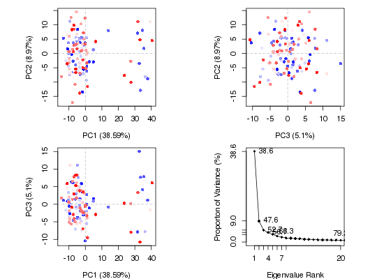
# Principal Component Analysis
pc <- pca.xyz(xyz[, ca.inds$xyz])
plot(pc, col = bwr.colors(nrow(xyz)))
pause()
Press ENTER/RETURN/NEWLINE to continue.
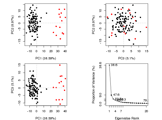
# Cluster in PC space
hc <- hclust(dist(pc$z[, 1:2]))
grps <- cutree(hc, k = 2)
plot(pc, col = grps)
pause()
Press ENTER/RETURN/NEWLINE to continue.
# Cross-Correlation Analysis
cij <- dccm(xyz[, ca.inds$xyz])
plot(cij)
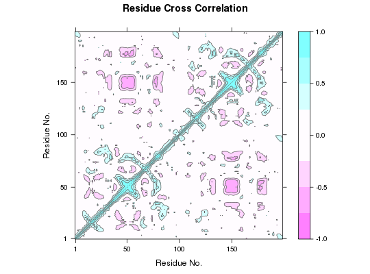
## view.dccm(cij, pdb, launch = TRUE)